The last post talked about the normal distribution and showed how to generate random numbers from that distribution by generating regular (uniform) random numbers and then counting the bits.

What would you do if you wanted to generate random numbers from a different, arbitrary distribution though? Let’s say the distribution is defined by a function even.

It turns out that in general this is a hard problem, but in practice there are a few ways to approach it. The below are the most common techniques for achieving this that I’ve seen.

• Inverting the CDF (analytically or numerically)
• Rejection Sampling
• Markov Chain Monte Carlo
• Ziggurat algorithm

This post talks about the first one listed: Inverting the CDF.

What Is A CDF?

The last post briefly explained that a PDF is a probability density function and that it describes the relative probability of numbers being chosen at random. A requirement of a PDF is that it has non negative value everywhere and also that the area under the curve is 1.

It needs to be non negative everywhere because a negative probability doesn’t make any sense. It needs to have an area under the curve of 1 because that means it represents the full 100% probability of all possible outcomes.

CDF stands for “Cumulative distribution function” and is related to the PDF.

A PDF is a function y=f(x) where y is the probability of the number x number being chosen at random from the distribution.

A CDF is a function y=f(x) where y is the probability of the number x, or any lower number, being chosen at random from that distribution.

You get a CDF from a PDF by integrating the PDF. From there you make sure that the CDF has a starting y value of 0, and an ending value of 1. You might have to do a bias (addition or subtraction) and/or scale (multiplication or division) to make that happen.

Why Invert the CDF? (And Not the PDF?)

With both a PDF and a CDF, you plug in a number, and you get information about probabilities relating to that number.

To get a random number from a specific distribution, we want to do the opposite. We want to plug in a probability and get out the number corresponding to that probability.

Basically, we want to flip x and y in the equation and solve for y, so that we have a function that does this. That is what we have to do to invert the CDF.

Why invert the CDF though and not the PDF? Check out the images below from Wikipedia. The first is some Gaussian PDF’s and the second is the same distributions as CDF’s:

The issue is that if we flip x and y’s in a PDF, there would be multiple y values corresponding to the same x. This isn’t true in a CDF.

Let’s work through sampling some PDFs by inverting the CDF.

Example 0: y=1

This is the easiest case and represents uniform random numbers, where every number is evenly likely to be chosen.

Our PDF equation is: where . The graph looks like this:

If we integrate the pdf to get the cdf, we get where which looks like this:

Now, to invert the cdf, we flip x and y, and then solve for y again. It’s trivially easy…

Now that we have our inverted CDF, which is , we can generate uniform random numbers, plug them into that equation as x and get y which is the actual value drawn from our PDF.

You can see that since we are plugging in numbers from an even distribution and not doing anything to them at all, that the result is going to an even distribution as well. So, we are in fact generating uniformly distributed random numbers using this inverted CDF, just like our PDF asked for.

This is so trivially simple it might be confusing. If so, don’t sweat it. Move onto the next example and you can come back to this later if you want to understand what I’m talking about here.

Note: The rest of the examples are going to have x in [0,1] as well but we are going to stop explicitly saying so. This process still works when x is in a different range of values, but for simplicity we’ll just have x be in [0,1] for the rest of the post.

Example 1: y=2x

The next easiest case for a PDF is which looks like this:

You might wonder why it’s instead of . This is because the area under the curve is 0.5. PDF’s need to have an area of 1, so I multiplied by 2 to make it have an area of 1.

What this PDF means is that small numbers are less likely to be picked than large numbers.

If we integrate the PDF to get the CDF, we get which looks like this:

Now let’s flip x and y and solve for y again.

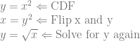
We now have our inverted CDF which is and looks like this:

Now, if we plug uniformly random numbers into that formula as x, we should get as output samples that follow the probability of our PDF.

We can use a histogram to see if this is really true. We can generate some random numbers, square root them, and count how many are in each range of values.

Here is a histogram where I took 1,000 random numbers, square rooted them, and put their counts into 100 buckets. Bucket 1 counted how many numbers were in [0, 0.01), bucket 2 counted how many numbers were in [0.01, 0.02) and so on until bucket 100 which counted how many numbers were in [0.99, 1.0).

Increasing the number of samples to 100,000 it gets closer:

At 1,000,000 samples you can barely see a difference:

The reason it doesn’t match up at lower sample counts is just due to the nature of random numbers being random. It does match up, but you’ll have some variation with lower sample counts.

Example 2: y=3x^2

Let’s check out the PDF . The area under that curve where x is in [0,1) is 1.0 and it’s non negative everywhere in that range too, so it’s a valid PDF.

Integrating that, we get for the CDF. Then we invert the CDF:

And here is a 100,000 sample histogram vs the PDF to verify that we got the right answer:

Example 3: Numeric Solution

So far we’ve been able to invert the CDF to get a nice easy function to transform uniform distribution random numbers into numbers from the distribution described by the PDF.

Sometimes though, inverting a CDF isn’t possible, or gives a complex equation that is costly to evaluate. In these cases, you can actually invert the CDF numerically via a lookup table.

A lookup table may also be desired in cases where eg you have a pixel shader that is drawing numbers from a PDF, and instead of making N shaders for N different PDFs, you want to unify them all into a single shader. Passing a lookup table via a constant buffer, or perhaps even via a texture can be a decent solution here. (Note: if storing in a texture you may be interested in fitting the data with curves and using this technique to store it and recall it from the texture: GPU Texture Sampler Bezier Curve Evaluation)

Let’s invert a PDF numerically using a look up table to see how that would work.

Our PDF will be:

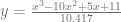
And looks like this:

It’s non negative in the range we care about and it integrates to 1.0 – or it integrates closely enough… the division by 10.417 is there for that reason, and using more digits would get it closer to 1.0.

What we are going to do is evaluate that PDF at N points to get a probability for those samples of numbers. That will give us a lookup table for our PDF.

We are then going to make each point be the sum of all the PDF samples to the left of it to make a lookup table for a CDF. We’ll also have to normalize the CDF table since it’s likely that our PDF samples don’t all add up (integrate) to 1.0. We do this by dividing every item in the CDF by the last entry in the CDF. If you look at the table after that, it will fully cover everything from 0% to 100% probability.

Below are some histogram comparisons of the lookup table technique vs the actual PDF.

Here is 100 million samples (to make it easier to see the data without very much random noise), in 100 histogram buckets, and a lookup table size of 3 which is pretty low quality:

Increasing it to a lookup table of size 5 gives you this:

Here’s 10:

25:

And here’s 100:

So, not surprisingly, the size of the lookup table affects the quality of the results!

Code

here is the code I used to generate the data in this post, which i visualized with open office. I visualized the function graphs using wolfram alpha.

#define _CRT_SECURE_NO_WARNINGS

#include 
#include 
#include 
#include 

template 
void Test (const char* fileName, const PDF_LAMBDA& PDF, const INVERSE_CDF_LAMBDA& inverseCDF)
{
    // seed the random number generator
    std::random_device rd;
    std::mt19937 rng(rd());
    std::uniform_real_distribution dist(0.0f, 1.0f);

    // generate the histogram
    std::array histogram = { 0 };
    for (size_t i = 0; i < NUM_TEST_SAMPLES; ++i)
    {
        // put a uniform random number into the inverted CDF to sample the PDF
        float x = dist(rng);
        float y = inverseCDF(x);

        // increment the correct bin on the histogram
        size_t bin = (size_t)std::floor(y * float(NUM_HISTOGRAM_BUCKETS));
        histogram[std::min(bin, NUM_HISTOGRAM_BUCKETS -1)]++;
    }

    // write the histogram and pdf sample to a csv
    FILE *file = fopen(fileName, "w+t");
    fprintf(file, "PDF, Inverted CDF\n");
    for (size_t i = 0; i < NUM_HISTOGRAM_BUCKETS; ++i)
    {
        float x = (float(i) + 0.5f) / float(NUM_HISTOGRAM_BUCKETS);
        float pdfSample = PDF(x);
        fprintf(file, "%f,%f\n",
            pdfSample,
            NUM_HISTOGRAM_BUCKETS * float(histogram[i]) / float(NUM_TEST_SAMPLES)
        );
    }
    fclose(file);
}

template 
void TestPDFOnly (const char* fileName, const PDF_LAMBDA& PDF)
{
    // make the CDF lookup table by sampling the PDF
    // NOTE: we could integrate the buckets by averaging multiple samples instead of just the 1. This bucket integration is pretty low tech and low quality.
    std::array CDFLookupTable;
    float value = 0.0f;
    for (size_t i = 0; i < LOOKUP_TABLE_SIZE; ++i)
    {
        float x = float(i) / float(LOOKUP_TABLE_SIZE - 1); // The -1 is so we cover the full range from 0% to 100%
        value += PDF(x);
        CDFLookupTable[i] = value;
    }

    // normalize the CDF - make sure we span the probability range 0 to 1.
    for (float& f : CDFLookupTable)
        f /= value;

    // make our LUT based inverse CDF
    // We will binary search over the y's (which are sorted smallest to largest) looking for the x, which is implied by the index.
    // I'm sure there's a better & more clever lookup table setup for this situation but this should give you an idea of the technique
    auto inverseCDF = [&CDFLookupTable] (float y) {

        // there is an implicit entry of "0%" at index -1
        if (y < CDFLookupTable[0])
        {
            float t = y / CDFLookupTable[0];
            return t / float(LOOKUP_TABLE_SIZE);
        }

        // get the lower bound in the lut using a binary search
        auto it = std::lower_bound(CDFLookupTable.begin(), CDFLookupTable.end(), y);

        // figure out where we are at in the table
        size_t index = it - CDFLookupTable.begin();

        // Linearly interpolate between the values
        // NOTE: could do other interpolation methods, like perhaps cubic (https://blog.demofox.org/2015/08/08/cubic-hermite-interpolation/)
        float t = (y - CDFLookupTable[index - 1]) / (CDFLookupTable[index] - CDFLookupTable[index - 1]);
        float fractionalIndex = float(index) + t;
        return fractionalIndex / float(LOOKUP_TABLE_SIZE);
    };

    // call the usual function to do the testing
    Test(fileName, PDF, inverseCDF);
}

int main (int argc, char **argv)
{
    // PDF: y=2x
    // inverse CDF: y=sqrt(x)
    {
        auto PDF = [] (float x) { return 2.0f * x; };
        auto inverseCDF = [] (float x) { return std::sqrt(x); };

        Test("test1_1k.csv", PDF, inverseCDF);
        Test("test1_100k.csv", PDF, inverseCDF);
        Test("test1_1m.csv", PDF, inverseCDF);
    }

    // PDF: y=3x^2
    // inverse CDF: y=cuberoot(x) aka y = pow(x, 1/3)
    {
        auto PDF = [] (float x) { return 3.0f * x * x; };
        auto inverseCDF = [](float x) { return std::pow(x, 1.0f / 3.0f); };

        Test("test2_100k.csv", PDF, inverseCDF);
    }

    // PDF: y=(x^3-10x^2+5x+11)/10.417
    // Inverse CDF Numerically via a lookup table
    {
        auto PDF = [] (float x) {return (x*x*x - 10.0f*x*x + 5.0f*x + 11.0f) / (10.417f); };
        TestPDFOnly("test3_100m_3.csv", PDF);
        TestPDFOnly("test3_100m_5.csv", PDF);
        TestPDFOnly("test3_100m_10.csv", PDF);
        TestPDFOnly("test3_100m_25.csv", PDF);
        TestPDFOnly("test3_100m_100.csv", PDF);
    }

    return 0;
}