Blue noise comes in two main flavors: sample points and masks. I’ll be calling blue noise masks “blue noise textures” in this post.

The code that accompanies this post, implementing the void and cluster algorithm, and running tests on it, can be found at:
https://github.com/Atrix256/VoidAndCluster

Update: Jonathan Dupuy has a GPU implementation that runs much more quickly than this CPU implementation. https://github.com/jdupuy/BlueNoiseDitherMaskTiles

Blue Noise Sample Points

Blue noise sample points can be used when you are taking samples for integration, like when sampling shadow maps, taking AO samples, or when doing path tracing. Blue noise doesn’t converge as fast as other sampling patterns, but it is really good at hiding error by evenly distributing it, as if error diffusion had been done.

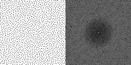
Here are some blue noise samples and their frequency magnitudes:

Here’s an example result of blue noise vs white noise sampling, from https://www.arnoldrenderer.com/research/dither_abstract.pdf

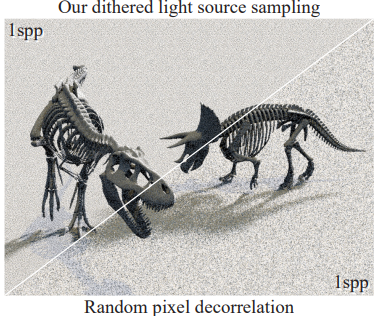
If you can afford enough samples to converge to the right result, you should do that, and you should use a sequence that converges quickly, such as Martin Robert’s R2 sequence (a generalization of the golden ratio, which is competitive with sobol!): http://extremelearning.com.au/unreasonable-effectiveness-of-quasirandom-sequences/

If you can’t afford enough samples to converge, that’s when you should reach for blue noise, to minimize the appearance of the error that will be in the resulting image.

To get blue noise samples, my go to method is “Mitchell’s Best Candidate Algorithm”:
https://blog.demofox.org/2017/10/20/generating-blue-noise-sample-points-with-mitchells-best-candidate-algorithm/

That algorithm is easy to understand and quick to implement, and while it makes decent results, it isn’t the best algorithm. The best blue noise sample point algorithms all seem to be based on capacity constrained Voronoi diagrams (CCVD). One benefit of Mitchell’s best candidate algorithm though is that the sample points it makes are progressive. That means if you generate 1024 sample points, using the first N of them for any N will still be blue noise. With CCVD algorithms, the sample points aren’t blue unless you use them all. This notion of progressive samples is something that will come up again in this post later on.

Blue Noise Textures

The second kind of blue noise is blue noise masks or textures.

One thing blue noise textures are good for is dithering data: adding random noise before quantization. Quantization lets you store data in fewer bits, and dithering before quantization gives a result that makes it harder (sometimes virtually impossible) to tell that it is even using fewer bits.

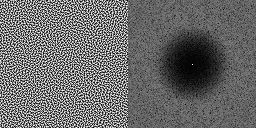
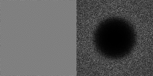
Here is a blue noise texture and it’s DFT

This is an example of white vs blue noise used for dithering, from http://johanneskopf.de/publications/blue_noise/

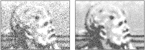
Using blue noise gives much better results than white noise, for the same amount of error. It does this by more evenly distributing the error, which gives results as if there was error diffusion done, without actually having to do the error diffusion step. The results are especially good when you animate the noise well. For more information on that, check out these posts of mine.
Part 1: https://blog.demofox.org/2017/10/31/animating-noise-for-integration-over-time/
Part 2: https://blog.demofox.org/2017/11/03/animating-noise-for-integration-over-time-2-uniform-over-time/

If that’s an area that you are interested in, you should give this a read too, making sure to check out the triangular distributed noise portion!

Click to access banding_in_games.pdf

Interestingly though, blue noise textures can also be used for sampling as this paper talks about: https://www.arnoldrenderer.com/research/dither_abstract.pdf

Here is another link between the two types of blue noise, where it shows how to turn blue noise textures into blue noise sample points of the desired density (like for making sample density be based on importance / the PDF): http://drivenbynostalgia.com/#frs

For blue noise textures, my go to has been to get them from this website where the author used the void and cluster algorithm to generate blue noise textures: http://momentsingraphics.de/?p=127

It’s been on my todo list for a while to understand and implement the void and cluster algorithm myself so that if that website ever goes down, I wouldn’t lose my only source of “the good stuff”. This post is the result of me finally doing that!

It’s possible to make blue noise (and other colors of noise too) by repeatedly filtering white noise: https://blog.demofox.org/2017/10/25/transmuting-white-noise-to-blue-red-green-purple/

Doing it that way has some problems though depending on what it is you want to use the blue noise for: https://blog.demofox.org/2018/08/12/not-all-blue-noise-is-created-equal/

Using Both Types of Blue Noise Together

I tend to use blue noise a lot in my rendering techniques, because it’s a nice way to get the look of higher sample counts (the appearance of low error), without spending the cost of higher sample counts.

It’s fairly common that I will use both types of blue noise together even!

For example, if I’m taking multiple PCF samples of a shadow map, I’ll make some blue noise sampling points to sample the shadow map per pixel. I’ll also use a 64×64 blue noise texture tiled across the screen as a per pixel random number for rotating those sample points per pixel.

As a bonus, i’ll use the golden ratio (conjugate) to make the noise be low discrepancy over time, as well as being blue over space by doing this after reading the value from the blue noise texture:

blueNoiseValue = fract(blueNoiseValue + 0.61803398875f * (frameNumber % 64));

The end result is really nice, and looks as though many more samples were taken than actually were.

(Beware: doing random sampling in cache friendly ways can be a challenge though)

Void And Cluster

The void and cluster algorithm was introduced in 1993 by Robert Ulichney and was previously under patent, but it seems to have expired into the public domain now.

Here is the paper:

Click to access 1993-void-cluster.pdf

The algorithm has four steps:

1. Generate Initial Binary Pattern – Make blue noise distributed sample points.
2. Phase 1 – Make those points progressive.
3. Phase 2 – Make more progressive sample points, until half of the pixels are sample points.
4. Phase 3 – Make more progressive sample points, until all pixels are sample points.

Since the points are progressive, it means they have some ordering to them. This is called their rank. The final blue noise texture image shades pixels based on their rank: lower numbers are darker, while higher numbers are brighter. The end goal is that you should have (as much as possible) an even number of each pixel value; you want a flat histogram.

Something interesting is that Phase 1 turns non progressive blue noise sample points into progressive blue noise sample points. I don’t know of any other algorithms to do this, and it might be common knowledge/practice, but it seems like this would be useful for taking CCVD blue noise sample points which are not progressive and making them progressive.

Before we talk about the steps, let’s talk about how to find voids and clusters.

Finding Voids and Clusters

Each step of this algorithm needs to identify the largest void and/or the tightest cluster in the existing sample points.

The tightest cluster is defined as the sample point that has the most sample points around it.

The largest void is defined as the empty pixel location that has the most empty pixel locations around it.

How the paper finds voids and clusters is by calculating a type of “energy” score for each pixel, where the energy goes up as it has more 1’s around it, and it goes up as they are closer to it.

Let’s say we are calculating the total energy for a pixel P.

To do that, we’ll loop through every pixel and calculate how much energy they contribute to pixel P. Add these all up and that is the energy of the pixel P.

If we are looking at how much energy a specific pixel S contributes to pixel P, we use this formula:

Energy= e^(-distanceSquared/(2*sigma*sigma))

The void and cluster paper uses a “sigma” of 1.5 which means the divisor 4.5. The “free blue noise textures” implementation uses a sigma of 1.9 and i have to agree that I think that sigma gives better results. A sigma of 1.9 makes the divisor be 7.22.

Distance squared is the squared distance between S and P, but using a “torroidal” wrap around distance which makes the resulting texture tileable as a side effect of satisfying “frequency space needs” of the pattern needing to be tileable. (I wrote a post about how to calculate torroidal distance if you are curious! https://blog.demofox.org/2017/10/01/calculating-the-distance-between-points-in-wrap-around-toroidal-space/)

Now that you know how to calculate an energy for each pixel, the hard part is done!

The pixel that has the highest total energy is the tightest cluster.

The pixel that has the lowest total energy is the largest void.

Generate Initial Binary Pattern

To start out, you need to make a binary pattern that is the same size as your output image, and has no more than half of the values being ones. In the code that goes with this post, I set 1/10th of the values to ones.

Then, in a loop you:

1) Find the tightest cluster and remove the one.
2) Find the largest void and put the one there.

You repeat this until the tightest cluster found in step 1 is the same largest void found in step 2.

After this, the initial binary pattern will be blue noise distributed sample points but they aren’t progressive because they have no sense of ordering.

This current binary pattern is called the “prototype binary pattern” in the paper.

Phase 1 – Make The Points Progressive

Phase 1 makes the initial binary pattern progressive, by giving a rank (an ordering) to each point.

To give them ranks you do this in a loop:

1) Find the tightest cluster and remove it.
2) The rank for that pixel you just removed is the number of ones left in the binary pattern.

Continue this until you run out of points.

Phase 2 – Make Progressive Points Until Half Are Ones

Phase 2 resets back to the prototype binary pattern and then repeatedly adds new sample points to it, until half of the binary pattern is ones.

It does this in a loop:

1) Find the largest void and insert a one.
2) The rank for the pixel you just added is the number of ones in the binary pattern before you added it.

Continue until half of the binary pattern is ones.

Phase 3 – Make Progressive Points Until All Are Ones

Phase 3 continues adding progressive sample points until the entire binary pattern is made up of ones.

It does this by reversing the meaning of zeros and ones in the energy calculation and does this in a loop:

1) Find the largest CLUSTER OF ZEROS and insert a one.
2) The rank for the pixel you just added is the number of ones in the binary pattern before you added it.

Continue until the entire binary pattern is ones.

You now have a binary pattern that is full of ones, and you should have a rank for every pixel. The last step is to turn this into a blue noise texture.

Finalizing The Texture

To make a blue noise texture, you need to turn ranks into pixel values.

If your output texture is 8 bits, that means you need to turn your ranks that are 0 to N, into values that are 0 to 255. You want to do this in a way where as much as possible, you have an even number of every value from 0 to 255.

I do this by multiplying the rank by 256 and dividing by the number of pixels (which is also the number of ranks there are).

Optimization Attempts

I tried a variety of optimizations on this algorithm. Some worked, some didn’t.

What I ultimately came to realize is that this algorithm is not fast, and that when you are using it, it’s because you want high quality results. Because of this, the optimizations really ought to be limited to things that don’t hurt the quality of the output.

For instance, if the algorithm takes 10 minutes to run, you aren’t going to shave off 30 seconds to get results that are any less good. You are running a ~10 minute algorithm because you want the best results you can get.

Success: Look Up Table

The best optimization I did by far was to use a look up table for pixel energy.

I made a float array the same size as the output, and whenever I put a 1 in the binary pattern, i also added that pixel’s energy into the energy look up table for all pixels. When removing a 1, i subtracted that pixel’s energy from the look up table for all pixels.

Using a look up table, finding the highest number is all it takes to find the tightest cluster, and finding the lowest number is all it takes to find the largest void.

I further sped this up by using threaded work to update the pixels.

I first used std::thread but didn’t get much of a win because there are a lot of calls to updating the LUT, and all the time moved from doing LUT calculation to thread creates and destroys. Switching to open mp (already built into visual studio’s compiler!) my perf got a lot better because open mp uses thread pools instead of creating/destroying threads each invocation.

Failure: Limiting to 3 Sigma

The equation to calculate pixel energy is actually a Gaussian function. Knowing that Gaussians have 99.7% of their value withing +/- 3 sigma, i decided to try only considering pixels within a 3*sigma radius when calculating the energy for a specific pixel.

While this tremendously sped up execution time, it was a failure for quality because pixels were blind to other pixels that were farther than 6 pixels away.

In the early and late stages of this blue noise generation algorithm, the existing sample points are pretty sparse (farther apart) and you are trying to add new points that are most far apart from existing points. If the farthest away you can see is 6 pixels, but your blue noise texture is 512×512, that means samples are not going to be very well distributed (blue noise distributed) at those points in time.

That had the result of making it so low and high threshold values used on the blue noise texture gave very poor results. (Thanks to Mikkel Gjoel for pointing out these edges to test for blue noise textures!)

Didn’t Try: DFT/IDFT for LUT

The “free blue noise textures” website implementation does a neat trick when it wants to turn a binary sample pattern into a look up table as I described it.

It does a DFT on the binary sample pattern, multiplies each pixel by the frequency space representation of a gaussian function of the desired size, and then does an inverse DFT to get the result as if convolution had been done. This uses the convolution theorem (a multiplication in frequency space is convolution in image space) to presumably get the LUT made faster.

I didn’t try this, but it doesn’t affect quality as far as I can tell (comparing my results to his), and i’m pretty sure it could be a perf win, but not sure by how much.

How I’ve written the code, there are two specific times that i want to make a LUT from scratch, but many, many more times i just want an incremental update to the LUT (at 1024×1024 that’s roughly 1 million LUT updates I would want to do) so i didn’t pursue this avenue.

Probable Success: Mitchell’s Best Candidate

Noticing the result of “initial binary pattern” and “phase 1” was to make a progressive blue noise sample, I thought it might be a good idea to replace those with an algorithm to directly make progressive blue noise samples.

I grabbed my goto algorithm and gave it a shot and it is noticeably faster, and seems to give decent results, but it also gives DIFFERENT results. The difference is probably harmless, but out of abundance of caution for correctness, I wouldn’t consider this a for sure success without more analysis.

Results

The code that goes with this post can be found at: https://github.com/Atrix256/VoidAndCluster

Speed

At 256×256, on my machine with my implementation, it took 400.2 seconds to run the standard void and cluster algorithm. Using Mitchell’s best candidate instead of the initial binary pattern and phase 1, it took 348.2 seconds instead. That’s a 13% savings in time.

At 128×128, standard void and cluster took 24.3 seconds, while the Mitchell’s best candidate version took 21.2 seconds. That’s a 13% time savings again.

At 64×64, it was 1.3 seconds vs 1.1 seconds which is about 13% time savings again.

Quality

From top to bottom is void and cluster, void and cluster using mitchell’s algorithm, and the bottom is a blue noise texture taken from the “free blue noise textures” site.

Here the same textures are, going through a “threshold” test to make sure they make good quality blue noise of every possible density. Same order: void and cluster, void and cluster using mitchell’s algorithm, and the bottom one is taken from the other website. You can definitely see a difference in the middle animation vs the top and bottom, so using the best candidate algorithm changes things, but it seems to be better at low sample counts and maybe not as good at low to medium sample counts. Hard to say for sure…

Red Noise

Lately I’ve been having a fascination with red noise as well.

Where blue noise is random values that have neighbors being very different from each other, red noise is random values that have neighbors that are close to each other.

Red noise is basically a “random walk”, but stateless. If you had a red noise texture, you could look some number of pixels forward and would get the position of the random walk that many steps away from your current position.

The simplest Markov Chain Monte Carlo algorithms use a random walk to do their work, but I’m not sure that a higher quality random walk would be very helpful there.

I’m sure there must be some usage case for red noise but I haven’t found it yet.

In any case, I do believe that the void and cluster algorithm could be adapted to generate red noise, but I’m not sure the specifics of how you’d do that.

If i figure it out, i’ll make a follow up post and link from here. If you figure it out, please share details!

Some more cool stuff regarding noise colors is coming to this blog, so be on the lookout 🙂