Hash tables are great in that you can hash a key and then use that hash as an index into an array to get the information associated with that key. That is very fast, so long as you use a fast hash function.
The story doesn’t end there though because hash functions can have collisions – multiple things can hash to the same value even though they are different. This means that in practice you have to do things like store a list of objects per hash value, and when doing a lookup, you need to do a slower full comparison against each item in the bucket to look for a match, instead of being able to only rely on the hash value comparisons.
What if our hash function didn’t have collisions though? What if we could take in N items, hash them, and get 0 to N-1 as output, with no collisions? This post will talk about how to make that very thing happen, with simple sample C++ code as well, believe it or not!
Minimal Perfect Hashing
Perfect hashing is a hash function which has no collisions. You can hash N items, and you get out N different hash values with no collisions. The number of items being hashed has to be smaller than or equal to the possible values your hash can give as output though. For instance if you have a 4 bit hash which gives 16 possible different hash values, and you hash 17 different items, you are going to have at least one collision, it’s unavoidable. But, if you hash 16 items or fewer, it’s possible in that situation that you could have a hash which had no collisions for the items you hashed.
Minimal perfect hashing takes this a step further. Not only are there no collisions, but when you hash N items, you get 0 to N-1 as output.
You might imagine that this is possible – because you could craft limitless numbers of hashing algorithms, and could pass any different salt value to it to change the output values it gives for inputs – but finding the specific hashing algorithm, and the specific salt value(s) to use sounds like a super hard brute force operation.
The method we are going to talk about today is indeed brute force, but it cleverly breaks the problem apart into smaller, easier to solve problems, which is pretty awesome. It’s actually a pretty simple algorithm too.
Here is how you create a minimal perfect hash table:
- Hash the items into buckets – there will be collisions at this point.
- Sort the buckets from most items to fewest items.
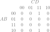
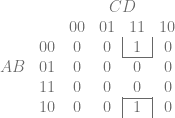
- Find a salt value for each bucket such that when all items in that bucket are hashed, they claim only unclaimed slots. Store this array of salt values for later. it will be needed when doing a data lookup.
- If a bucket only has one item, instead of searching for a salt value, you can just find an unclaimed index and store -(index+1) into the salt array.
Once you have your minimal perfect hash calculated, here is how you do a lookup:
- Hash the key, and use that hash to find what salt to use.
- If the salt is positive (or zero), hash the key again using the salt. The result of that hash will be an index into the data table.
- If the salt is negative, take the absolute value and subtract one to get the index in the data table.
- Since it’s possible the key being looked for isn’t in the table, compare the key with the key stored at that index in the table. If they match, return the data at that index. If they don’t match, the key was not in the table.
Pretty simple isn’t it?
Algorithm Characteristics
This perfect minimal hash algorithm is set up to be slow to generate, but fast to query. This makes it great for situations where the keys are static and unchanging, but you want fast lookup times – like for instance loading a data file for use in a game.
Interestingly though, while you can’t add new keys, you could make it so you could delete keys. You would just remove the key / value pair from the data set, and then when doing a lookup you’d find an empty slot.
Also, there is nothing about this algorithm that says you can’t modify the data associated with the keys, at runtime. Modifying the data associated with a key doesn’t affect where the key/value pair is stored in the table, so you can modify the data all you want.
If you wanted to be able to visit the items in a sorted order, when searching for the perfect minimal hash, you could also make the constraint that when looking for the salt values, that not only did the items in the bucket map to an unclaimed slot, you could make sure they mapped to the correct slot that they should be in to be in sorted order. That would increase the time it took to generate the table, and increase the chances that there was no valid solution for any salt values used, but it is possible if you desire being able to know the items in some sorted order.
Interestingly, the generation time of the minimal perfect hash apparently grows linearly with the number of items it acts on. That makes it scale well. On my own computer for instance, I am able to generate the table for 100,000 items in about 4.5 seconds.
Also, in my implementation, if you have N items, it has the next lower power of two number of salt values. You could decrease the number of salt values used if you wanted to use less memory, but that would again come at the cost of increased time to generate the table, as well as increase the chances that there was no valid solution for any salt values used.
Example Code
Below is a simple implementation of the algorithm described.
The main point of the code (besides functionality) is readability so it isn’t optimized as well as it could be, but still runs very fast (100,000 items processed in about 4.5 seconds on my machine). Debug is quite a bit slower than release for me though – I gave up on those same 100,000 items after a few minutes running in debug.
The code below uses MurmurHash2, but you could drop in whatever hashing algorithm you wanted.
The data file for this code is words.txt and comes to us courtesy of English Wordlists.
#include <vector>
#include <algorithm>
#include <assert.h>
#include <fstream>
#include <string>

unsigned int MurmurHash2(const void * key, int len, unsigned int seed);

//=================================================================================
template <typename VALUE>
class CPerfectHashTable {
public:

    typedef std::pair<std::string, VALUE> TKeyValuePair;
    typedef std::vector<TKeyValuePair> TKeyValueVector;
    struct SKeyValueVectorBucket {
        TKeyValueVector m_vector;
        size_t          m_bucketIndex;
    };
    typedef std::vector<struct SKeyValueVectorBucket> TKeyValueVectorBuckets;

    // Create the perfect hash table for the specified data items
    void Calculate (const TKeyValueVector& data) {

        // ----- Step 1: hash each data item and collect them into buckets.
        m_numItems = data.size();
        m_numBuckets = NumBucketsForSize(m_numItems);
        m_bucketMask = m_numBuckets - 1;
        m_salts.resize(m_numBuckets);
        m_data.resize(m_numItems);
        TKeyValueVectorBuckets buckets;
        buckets.resize(m_numBuckets);

        for (size_t i = 0; i < m_numBuckets; ++i)
            buckets[i].m_bucketIndex = i;

        for (const TKeyValuePair& pair : data) {
            size_t bucket = FirstHash(pair.first.c_str());
            buckets[bucket].m_vector.push_back(pair);
        }

        // ----- Step 2: sort buckets from most items to fewest items
        std::sort(
            buckets.begin(),
            buckets.end(),
            [](const SKeyValueVectorBucket& a, const SKeyValueVectorBucket& b) {
                return a.m_vector.size() > b.m_vector.size();
            }
        );

        // ----- Step 3: find salt values for each bucket such that when all items
        // are hashed with their bucket's salt value, that there are no collisions.
        // Note that we can stop when we hit a zero sized bucket since they are sorted
        // by length descending.
        std::vector<bool> slotsClaimed;
        slotsClaimed.resize(m_numItems);
        for (size_t bucketIndex = 0, bucketCount = buckets.size(); bucketIndex < bucketCount; ++bucketIndex) {
            if (buckets[bucketIndex].m_vector.size() == 0)
                break;
            FindSaltForBucket(buckets[bucketIndex], slotsClaimed);
        }
    }

    // Look up a value by key.  Get a pointer back.  null means not found.
    // You can modify data if you want, but you can't add/remove/modify keys without recalculating.
    VALUE* GetValue (const char* key) {

        // do the first hash lookup and get the salt to use
        size_t bucket = FirstHash(key);
        int salt = m_salts[bucket];

        // if the salt is negative, it's absolute value minus 1 is the index to use.
        size_t dataIndex;
        if (salt < 0)
            dataIndex = (size_t)((salt * -1) - 1);
        // else do the second hash lookup to get where the key value pair should be
        else
            dataIndex = MurmurHash2(key, strlen(key), (unsigned int)salt) % m_data.size();

        // if the keys match, we found it, else it doesn't exist in the table
        if (m_data[dataIndex].first.compare(key) == 0)
            return &m_data[dataIndex].second;
        return nullptr;
    }

private:

    unsigned int FirstHash (const char* key) {
        return MurmurHash2(key, strlen(key), 435) & m_bucketMask;
    }

    void FindSaltForBucket (const SKeyValueVectorBucket& bucket, std::vector<bool>& slotsClaimed) {

        // if the bucket size is 1, instead of looking for a salt, just encode the index to use in the salt.
        // store it as (index+1)*-1 so that we can use index 0 too.
        if (bucket.m_vector.size() == 1) {
            for (size_t i = 0, c = slotsClaimed.size(); i < c; ++i)
            {
                if (!slotsClaimed[i])
                {
                    slotsClaimed[i] = true;
                    m_salts[bucket.m_bucketIndex] = (i + 1)*-1;
                    m_data[i] = bucket.m_vector[0];
                    return;
                }
            }
            // we shouldn't ever get here
            assert(false);
        }

        // find the salt value for the items in this bucket that cause these items to take
        // only unclaimed slots
        for (int salt = 0; ; ++salt) {
            // if salt ever overflows to a negative number, that's a problem.
            assert(salt >= 0);
            std::vector<size_t> slotsThisBucket;
            bool success = std::all_of(
                bucket.m_vector.begin(),
                bucket.m_vector.end(),
                [this, &slotsThisBucket, salt, &slotsClaimed](const TKeyValuePair& keyValuePair) -> bool {
                    const char* key = keyValuePair.first.c_str();
                    unsigned int slotWanted = MurmurHash2(key, strlen(key), (unsigned int)salt) % m_numItems;
                    if (slotsClaimed[slotWanted])
                        return false;
                    if (std::find(slotsThisBucket.begin(), slotsThisBucket.end(), slotWanted) != slotsThisBucket.end())
                        return false;
                    slotsThisBucket.push_back(slotWanted);
                    return true;
                }
            );

            // When we find a salt value that fits our constraints, remember the salt
            // value and also claim all the buckets.
            if (success)
            {
                m_salts[bucket.m_bucketIndex] = salt;
                for (size_t i = 0, c = bucket.m_vector.size(); i < c; ++i)
                {
                    m_data[slotsThisBucket[i]] = bucket.m_vector[i];
                    slotsClaimed[slotsThisBucket[i]] = true;
                }
                return;
            }
        }
    }

    static size_t NumBucketsForSize (size_t size) {
        // returns how many buckets should be used for a specific number of elements.
        // Just uses the power of 2 lower than the size, or 1, whichever is bigger.
        if (!size)
            return 1;

        size_t ret = 1;
        size = size >> 1;
        while (size) {
            ret = ret << 1;
            size = size >> 1;
        }
        return ret;
    }

    // When doing a lookup, a first hash is done to find what salt to use
    // for the second hash.  This table stores the salt values for that second
    // hash.
    std::vector<int> m_salts;

    // NOTE: this stores both the key and the value.  This is to handle the
    // situation where a key is searched for which doesn't exist in the table.
    // That key will still hash to some valid index, so we need to detect that
    // it isn't the right key for that index.  If you are never going to look for
    // nonexistant keys, then you can "throw away the keys" and only store the
    // values.  That can be a nice memory savings.
    std::vector<TKeyValuePair> m_data;

    // useful values
    size_t m_numItems;
    size_t m_numBuckets;
    size_t m_bucketMask;
};

// MurmurHash code was taken from https://sites.google.com/site/murmurhash/
//=================================================================================
// MurmurHash2, by Austin Appleby

// Note - This code makes a few assumptions about how your machine behaves -

// 1. We can read a 4-byte value from any address without crashing
// 2. sizeof(int) == 4

// And it has a few limitations -

// 1. It will not work incrementally.
// 2. It will not produce the same results on little-endian and big-endian
//    machines.

unsigned int MurmurHash2 ( const void * key, int len, unsigned int seed )
{
    // 'm' and 'r' are mixing constants generated offline.
    // They're not really 'magic', they just happen to work well.

    const unsigned int m = 0x5bd1e995;
    const int r = 24;

    // Initialize the hash to a 'random' value

    unsigned int h = seed ^ len;

    // Mix 4 bytes at a time into the hash

    const unsigned char * data = (const unsigned char *)key;

    while(len >= 4)
    {
        unsigned int k = *(unsigned int *)data;

        k *= m;
        k ^= k >> r;
        k *= m;

        h *= m;
        h ^= k;

        data += 4;
        len -= 4;
    }

    // Handle the last few bytes of the input array

    switch(len)
    {
    case 3: h ^= data[2] << 16;
    case 2: h ^= data[1] << 8;
    case 1: h ^= data[0];
            h *= m;
    };

    // Do a few final mixes of the hash to ensure the last few
    // bytes are well-incorporated.

    h ^= h >> 13;
    h *= m;
    h ^= h >> 15;

    return h;
}


//=================================================================================
void WaitForEnter ()
{
    printf("Press Enter to quit");
    fflush(stdin);
    getchar();
}

//=================================================================================
int main (int argc, char **argv)
{
    // Read the data entries from a file.  Use the line as the key, and the line
    // number as the data.  Limit it to 100,000 entries.
    printf("Loading Data...");
    CPerfectHashTable<int> table;
    decltype(table)::TKeyValueVector data;
    std::ifstream file("words.txt");
    std::string str;
    int i = 0;
    while (std::getline(file, str) && i < 100000)
    {
        data.push_back(std::make_pair(str, i));
        ++i;
    }
    printf("Donenn");

    // make the perfect hash table
    printf("Generating Minimal Perfect Hash Table...");
    table.Calculate(data);
    printf("Donenn");

    // Verify results
    printf("Verifying results...");
    for (decltype(table)::TKeyValuePair& keyValuePair : data) {
        int* value = table.GetValue(keyValuePair.first.c_str());
        assert(value != nullptr);
        if (value == nullptr)
        {
            printf("Error, could not find data for key "%s"n", keyValuePair.first.c_str());
            WaitForEnter();
            return 0;
        }
        assert(*value == keyValuePair.second);
        if (*value != keyValuePair.second)
        {
            printf("  table["%s"] = %in", keyValuePair.first.c_str(), *value);
            printf("Incorrect value detected, should have gotten %i!n", keyValuePair.second);
            WaitForEnter();
            return 0;
        }
    }
    printf("Donenn");

    WaitForEnter();
    return 0;
}
Links & More
I learned the details of this algorithm from this page: Steve Hanov’s Blog: Throw away the keys: Easy, Minimal Perfect Hashing, after hearing about the technique mentioned occasionally by colleagues.
There are other ways to do minimal perfect hashing however. For instance give this a read: Minimal Perfect Hashing
One place that method is better than this one, is that in this one, when doing a lookup you have to hash the key twice. In the technique described by the last technique, you only have to hash the key once, and use that hash to combine the results of two lookups. The two lookups are not dependant so can be re-ordered or happen concurrently, which makes it faster on modern CPUs.
Apparently there are also some techniques for generating the minimal perfect hash on a large number of items by breaking them apart into smaller sets, which can then be paralelized across threads.
I also wanted to mention that a large part of the in memory representation of this data structure can come from storing the keys along with the data, to verify that you have indeed found the item you are looking for after doing the O(1) lookup. If you are in a situation where you are only ever going to be searching for keys that you know are in the table, you can actually forgo storing the keys, to bring the memory requirements down a significant amount.
Also, The example code implements this as a hash table, but you could also use this as a set, if you wanted fast membership tests. You could either store the keys, to be able to resolve when things were not part of the set, or, you could make a hash table of string to bool, where the bool specified whether something was in the set. Which one is better depends on your specific needs and whether you plan to search for unknown keys or not.
Lastly, as a byproduct of using a data structure like this, you can get a unique ID per key, which is the index that it appears in the data array. This can be super helpful if you have something like a list of filenames, where you would rather work with integers instead of specific file names, since integers are quicker and easier to compare, copy around, etc.
You could even make this data structure support lookups by either key or by unique id. This way, you could do a by key lookup the first time you needed to find something, and then could store off the ID to get it by ID from then on for a faster lookup. Heck, you could even do all your lookups “offline” (at tool time, not when the app is running) and for instance convert all file references in data files to be the each file’s unique ID instead. Then, you could toss out the keys of your data structure, only storing an array of data, and using the unique file ID to look into that table whenever you wanted to read or write meta data associated with that file. That would make lookups faster, and also decrease the memory requirements of memory resident data files.
It’s pretty cool stuff, and a pretty useful algorithm. Hopefully you find it useful as well (:
Update – 12/22/15
Interestingly, this post has had something like 15,000 readers since it was posted. That is by far the most read post on this blog 😛
Anyways, I wanted to add some more info I’ve found recently.
Here are three tools for doing minimal perfect hashing that are very likely to give you better results than the algorithm I describe above:
Here’s a conversation talking about gperf and the alternative applications, and pros and cons for each:
Stack Overflow: Making a perfect hash (all consecutive buckets full), gperf or alternatives?
Here’s a research paper on gperf by Doug Schmidt: GPERF – A Perfect Hash Function Generator
I had a thought that maybe there was some play here by using “logical synthesis” to come up with some algorithm to map the inputs (the keys of the hash table) to the outputs (collision free output indices).
I started looking into Karnaugh maps and then the Quine–McCluskey algorithm, and then espresso and espresso-exact (mincov). Where the first two things are decent at solving multi bit input to single bit output, the second two things are decent at solving multi bit input to multi bit output, allowing operations to be shared among bits.
While I haven’t found anyone using those specific algorithms to solve the problem, people have, and definitely are still, trying to also look into the ability to generate code without lookups. From what I’ve read so far, it sounds like finding such a function takes a lot longer to find and also that it runs more slowly in practice than a less perfect solution which has lookups.
Either way, this is still an active area of research, and plenty of folks are working on it so I’m going to leave it to them.
I also sort of have the feeling that if you are in need of minimal perfect hashing, you may be “doing it wrong”. For instance, if you are at all able to, you probably are likely to be better off having a pre-agreed on set of unique IDs per “thing” you want to look up. These unique IDs can be used directly as array indices for the magical always O(1) lookup that minimal perfect hashing is going for, and is actually a quicker lookup in practice since you don’t need to jump through special hoops to calculate the array index.
The only exceptions I can think of are:
- Real world requirements and not being able to reach the ideal situation – this is the boat I’m in right now. Ideally, systems would be asking about things by an integer ID, but I can’t get there in a single step, so the perfect hashing is a temporary bridge til I can get there.
- Even with IDs, sparse arrays are still problematic. You may have an ID per file that could be asked about, but say that you have 1,000,000 files, but you want to make an array of data for only 10,000 of them. How do you take the unique ID of a file and do a lookup into that smaller table? Minimal perfect hashing seems to be useful in this situation, but there may be other decent or comparable alternatives if you are already using integer IDs.