Calculating the Similarity of Histograms or PDFs & Interpolating Them Using the p-Wasserstein Distance

The code that goes with this post is at https://github.com/Atrix256/OT1D.

The title of this post is a mouthful but the topic is pretty useful.

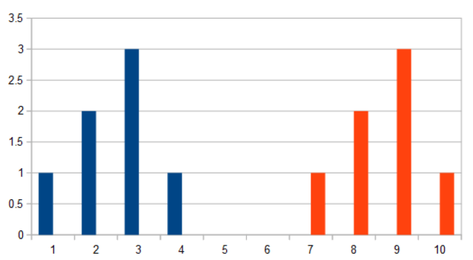
Let’s say that we have two histograms:

  • 1,2,3,1,0,0,0,0,0,0
  • 0,0,0,0,0,0,1,2,3,1

When you want to see how similar two histograms are, some common ways are:

  1. Treat the histograms as high dimensional vectors and dot product them. Higher values mean more similar.
  2. Treat the histograms as high dimensional points and calculate the distance between them, using the regular distance formula (aka L2 norm or Euclidian norm), taxi cab distance (aka L1 norm) or others. Lower values mean more similar.

Those aren’t bad methods, but they aren’t always the right choice depending on your needs.

  1. If you dot product these histograms as 10 dimensional vectors, you get a value of zero because there’s no overlap. If there are more or fewer zeros between them, you still get zero. This gives you no idea how similar they are other than they don’t overlap.
  2. If you calculate the distance between these 10 dimensional points, you will get a non zero value which is nice, but adding or removing zeros between them, the value doesn’t change. You can see this how the length of the vector (1,0,1) is the square root of 2, which is also the length of the vector (1,0,0,1) and (1,0,0,0,1). It doesn’t tell you really how close they are on the x axis.

In this case, let’s say we want a similarity metric where if we separate these histograms with more zeros, it tells us that they are less similar, and if we remove zeros or make them overlap, it tells us that they are more similar.

This is what the p-Wasserstein distance gives us. When we interpolate along this distance metric from the first histogram to the second, the first histogram slides to the right, and this is actually 1D optimal transport. This is in contrast to us just linearly interpolating the values of these histograms, where the first histogram would shrink as the second histogram grew.

The title of this post says that we will be working with both histograms and PDFs (probability distribution functions). A PDF is sort of like a continuous version of a histogram, but integrates to 1 and is limited to non negative values. In fact, if a histogram has only non negative values, and sums up to 1, it can be regarded as a PMF, or probability mass function, which is the discrete version of a PDF and is used for things like dice rolls, coin flips, and other discrete valued random events.

You can do similar operations with PDFs as you can with histograms to calculate similarity.

  1. Instead of calculating a dot product between vectors, you take the integral of the product of the two functions. Higher values means more similar, like with dot product. \int_0^1 f(x)g(x) \, dx. This is a a kind of continuous dot product.
  2. Instead of calculating a distance between points, you take the integral of the absolute value of the difference of the two functions raised to some power and then the result taken to one over the same power (\int_0^1 \left| f(x) - g(x) \right| ^n\, dx)^{1/n}. Lower values means more similar, like with distance. This is a kind of continuous distance calculation.

Also, any function that doesn’t have negative y values can be normalized to integrate to 1 over a range of x values and become a PDF. So, when we talk about PDFs in this post, we are really talking about any function that doesn’t have negative values over a specific range.

p-Wasserstein Distance Formula

“Optimal Transport: A Crash Course” by Kolouri et. al (https://www.imagedatascience.com/transport/OTCrashCourse.pdf) page 46 says that you can calculate p-Wasserstein distance like this (they use different symbols):

(\int_0^1 \left| F^{-1}(x) - G^{-1}(x) \right| ^p \, dx)^{1/p}

That looks a bit like the continuous distance integral we saw in the last section, but there are some important differences.

Let me explain the symbols in this function. First is p which is where the p in p-Wasserstein distance comes from. It can be 1, 2, 1.5, or any other number. If using the value 2, you’d call it 2-Wasserstein distance, and it would be dealing with the squares of differences between these functions F^{-1}(x) and G^{-1}(x).

Let’s say that we have a PDF called f. We can integrate that to get a CDF or cumulative distribution function that we’ll call F. We can then switch x and y and solve for y to get the inverse of that function, or F^{-1}. If we have another PDF called g, we can follow the same process to get G^{-1}.

When we calculate the integral above, either analytically / symbolically if we are able, or numerically otherwise, we get the p-Wasserstein distance which has the nice properties we described before.

A fun tangent: if you have the inverse CDF of a PDF, you can plug in a uniform random number in [0,1] to the inverse CDF and get a random number drawn from the original PDF. It isn’t always possible or easy to get the inverse CDF of a PDF, but this also works numerically – you can make a table out of the PDF, make a table for the CDF, and make a table for the inverse CDF from that, and do the same thing. More info on all of that at https://blog.demofox.org/2017/08/05/generating-random-numbers-from-a-specific-distribution-by-inverting-the-cdf/.

Calculating 2-Wasserstein Distance of Simple PDFs

Let’s start off by calculating some inverse CDFs of simple PDFs, then we’ll use them in the formula for calculating 2-Wasserstein distances.

Uniform PDF

First is the PDF y=1, which is for uniform random values. It integrates to 1 for x between 0 and 1 and is positive in that range as well.

If we integrate that to get the CDF, we get y=x.

If we flip x and y, and solve again for y to get the inverse CDF, we get y=x.

Linear PDF

The next PDF is y=2x. It integrates to 1 for x between 0 and 1 and is positive in that range as well.

If we integrate that, the CDF is y=x^2.

Flipping x and y and solving for y gives us the inverse CDF y=\sqrt{x}.

Quadratic PDF

The last PDF is y=3x^2. It integrates to 1 for x between 0 and 1 and is positive in that range as well.

If we integrate that, the CDF is y=x^3

Flipping x and y and solving for y gives us the inverse CDF y=\sqrt[3]{x}.

2-Wasserstein Distance From Uniform to Linear

The 2-Wasserstein distance formula looks like this:

(\int_0^1 \left| F^{-1}(x) - G^{-1}(x) \right| ^2 \, dx)^{1/2}

Let’s square the function for now and we’ll square root the answer later. Let’s also replace F^{-1} with the uniform PDF inverse CDF, and replace G^{-1} with the linear PDF inverse CDF. We can drop the absolute value since the square does that for us.

\int_0^1 (x - \sqrt{x})^2 \, dx

Expanding the equation, we get:

\int_0^1 x^2 -2x \sqrt{x} + x  \, dx

Luckily we can break that integral up into 3 integrals:

\int_0^1 x^2 \, dx - \int_0^1 2x \sqrt{x}\, dx + \int_0^1 x  \, dx

https://www.wolframalpha.com/ comes to the rescue here where you can ask it “integrate y=x^2 from 0 to 1” etc to get the answer to each integral.

1/3 - 4/5 +1/2 = 1/30

Remembering that we removed the square root from the formula at the beginning, we have to square root this to get our real answer.

\sqrt{1/30} = \sqrt{30}/30 = 0.18257418583

2-Wasserstein Distance From Uniform to Quadratic

We can do this again measuring the distance between uniform and quadratic.

\int_0^1 (x - \sqrt[3]{x})^2 \, dx

\int_0^1 x^2-2 x \sqrt[3]{x} + \sqrt[3]{x}^2 \, dx

1/3 - 6/7 +3/5 = 8/105

Square rooting that gives:

\sqrt{8/105} = (2 * \sqrt{210})/105 = 0.27602622373

2-Wasserstein Distance From Linear to Quadratic

We can do this again between linear and quadratic.

\int_0^1 (\sqrt{x} - \sqrt[3]{x})^2 \, dx

\int_0^1 x - 2 \sqrt{x} \sqrt[3]{x} + \sqrt[3]{x}^2 \, dx

1/2 - 12/11 + 3/5 = 1/110

Square rooting that gives:

\sqrt{110}/110 = 0.09534625892

These results tell us that uniform and quadratic are most different, and that linear and quadratic are most similar. Uniform and linear are in the middle. That matches what you’d expect when looking at the graphs.

Calculating p-Wasserstein Distance of More Complicated PDFs

If you have a more complex PDF that you can’t make an inverted CDF of, you can still calculate the distance metric numerically.

You start off by making a table of PDF values at evenly spaced intervals, then divide all entries by the sum of all entries to make it a tabular form of the PDF (it sums to 1). You then make a CDF table where each entry is the sum of PDF values at or before that location.

Now to evaluate the inverted CDF for a value x, you can do a binary search of the CDF table to find where that value x is. You also calculate what percentage the value is between the two indices it’s between so that you have a better approximation of the inverted CDF value. Alternately to a binary search, you could make an ICDF table instead.

If that sounds confusing, just imagine you have an array where the x axis is the array index and the y axis is the value in the array. This is like a function where if you have some index you can plug in as an x value, it gives you a y axis result. That is what the CDF table is. If you want to evaluate the inverted CDF or ICDF, you have a y value, and you are trying to find what x index it is at. Since the y value may be between two index values, you can give a fractional index answer to make the ICDF calculation more accurate.

Now that you can make an inverted CDF table of any PDF, we can use Monte Carlo integration to calculate our distance metric.

Let’s look at the formula again:

(\int_0^1 \left| F^{-1}(x) - G^{-1}(x) \right| ^p \, dx)^{1/p}

To calculate the inner integral, we pick a bunch of x values between 0 and 1, plug them into the equation and average the results that come out. After that, we take the answer to the 1/p power to get our final answer. The more samples you take of x, the more accurate the answer is.

\text{result}^p = \int_0^1 \left| F^{-1}(x) - G^{-1}(x) \right| ^p \, dx

Here is some C++ that implements that, with the ICDF functions being template parameters so you can pass any callable thing in (lambda, function pointer, etc) for evaluating the ICDF.

template <typename ICDF1, typename ICDF2>
float PWassersteinDistance(float p, const ICDF1& icdf1fn, const ICDF2& icdf2fn, int numSamples = 10000000)
{
    // https://www.imagedatascience.com/transport/OTCrashCourse.pdf page 45
    // Integral from 0 to 1 of abs(ICDF1(x) - ICDF2(x))^p
    // Then take the result to ^(1/p)
    double ret = 0.0;
    for (int i = 0; i < numSamples; ++i)
    {
        float x = RandomFloat01();
        float icdf1 = icdf1fn(x);
        float icdf2 = icdf2fn(x);
        double y = std::pow(std::abs((double)icdf1 - (double)icdf2), p);
        ret = Lerp(ret, y, 1.0 / double(i + 1));
    }
    return (float)std::pow(ret, 1.0f / p);
}

If both ICDFs are tables, that means they are both piecewise linear functions. You can get a noise free, deterministic calculation of the integral by integrating the individual sections of the tables, but the above is a generic way that will work for any (and mixed) methods for evaluating ICDFs.

Below is a table of the 2-Wasserstein distances calculated different ways. The analytic truth column is what we calculated in the last section and is the correct answer. The numeric function column is us running the above numerical integration code, using the inverted CDF we made symbolically in the last section. The last column “numeric table” is where we made a tabular inverted CDF by taking 10,000 PDF samples and making a 100 entry CDF, then using binary search to do inverse CDF evaluations.

Analytic TruthNumeric FunctionNumeric Table
Uniform To Linear0.182574185830.1825680.182596
Uniform To Quadratic0.276026223730.2760120.275963
Linear To Quadratic0.095346258920.0953270.095353

For kicks, here are p values of 1 and 3 to compare against 2. Calculated using the “numeric table” method.

123
Uniform To Linear0.1666090.1825960.192582
Uniform To Quadratic0.2499330.2759630.292368
Linear To Quadratic0.0833080.0953530.103187

Calculating p-Wasserstein Distance of PMFs

If you have a random variable with discrete random values – like a coin toss, or the roll of a 6 sided dice – you start with a PMF (probability mass function) instead of a PDF. A PMF says how likely each discrete event is, and all the events add up to 1.0. The PMF is probably already a table. You can then turn that into a CDF and continue on like we did in the last section. Let’s see how to make a CDF for a PMF.

When you evaluate y=CDF(x), the y value you get is the probability of getting the value x or lower. When you turn a PMF into a CDF, since it’s discrete, you end up with a piecewise function.

For instance, here is the the PMF 0.1, 0.3, 0.2, 0.4.

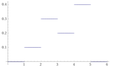
The CDF is 0.1, 0.4, 0.6, 1.0.

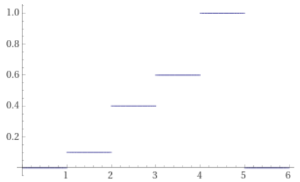
With a CDF you can now do the same steps as described in the last section.

Interpolating PDFs & Other Functions

Interpolating over p-Wassertstein distance is challenging in the general case. I’m going to dodge that for now, and just show the nice and easy way to interpolate over 1-Wasserstein distance.

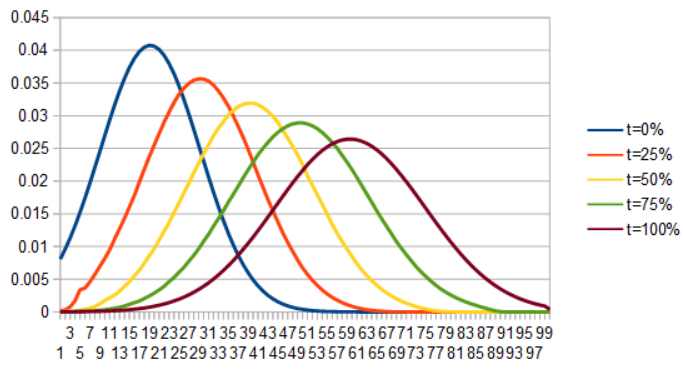
First let’s see what happens if we interpolate two gaussian PDFs directly… by linearly interpolating PDF(x) for each x to make a new PDF. As you can see, the gaussian on the left shrinks as the gaussian on the right grows.

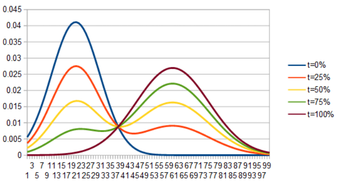
If we instead lerp ICDF(x) for each x to make a new ICDF, invert it to make a CDF, then differentiate it to get a PDF, we get this very interesting optimal transport interpolation:

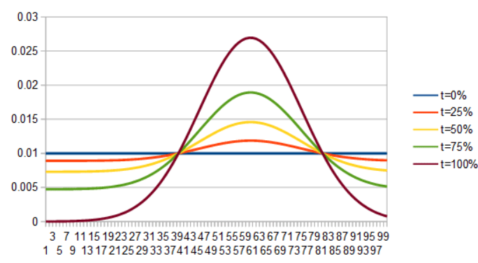
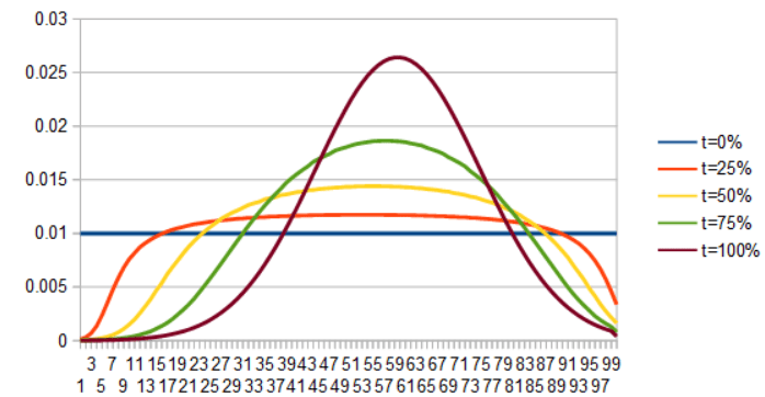
For a second example here is a uniform PDF interpolating into Gaussian, by lerping the PDFs and then the ICDFs.

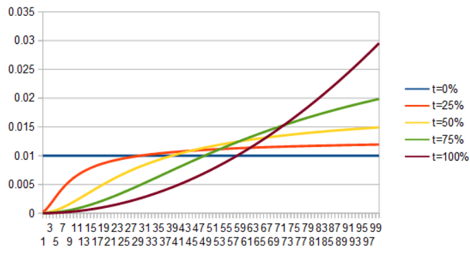
As a last set of examples, here is uniform to quadratic. First by lerping the PDFs, then by lerping the ICDFs.

It sounds like a lot of work interpolating functions by integrating the PDFs or PMFs to CDFs, inverting them to ICDFs, lerping, then inverting and differentiating, and it really is a lot of work.

However, like I mentioned before, if you a plug a uniform random value into an ICDF function, it will give you an unbiased random value from the PDF. This means that in practice, if you are generating non uniform random numbers, you often have an ICDF handy for the distribution already; either symbolically or numerically in a table. That makes this whole process a lot simpler: plug your uniform random x value into the two ICDFs, and return the result of lerping them. That’s all there is to it to generate random numbers that are from a PDF interpolated over 1-Wasserstein distance. That is extremely simple and very runtime friendly for graphics and game dev people. Again, more simply: just generate 2 random numbers and interpolate them.

If you are looking for some intuition as to why interpolating the ICDF does what it does, here are some bullet points.

  • PDF(x) or PMF(x) tells you how probable x is.
  • CDF(x) tells you how probable it is to get the value x or lower.
  • ICDF(x) tells you the value you should get, for a uniform random number x.
  • Interpolating PDF1(x) to PDF2(x) makes the values in PDF1 less likely and the values in PDF2 more likely. It’s shrinking PDF1 on the graph, and growing PDF2.
  • Interpolating CDF1(x) to CDF2(x) gets the values that the two PDFs would give you for probability x, and interpolates between them. If a random roll would get you a 3 from the first PDF, and a 5 from the second PDF, this interpolates between the 3 and the 5.

In this section we’ve talked about linear interpolation between two PDFs, but this can actually be generalized.

  1. A linear interpolation is just a degree 1 (linear) Bezier curve, which has 2 control points that are interpolated between. The formula for a linear Bezier curve is just A(1-t)+Bt which looks exactly like linear interpolation, because it is! With a quadratic Bezier curve, you have 3 control points, which means you could have three probability distributions you were interpolating between, but it would only pass through the two end points – the middle PDF would never be fully used, it would just influence the interpolation. You can do cubic and higher as well for more PDFs to interpolate between. Check this out for more info about Bezier curves. https://blog.demofox.org/2015/05/25/easy-binomial-expansion-bezier-curve-formulas/.
  2. A linear interpolation is a Bezier curve on a one dimensional 1-simplex aka a line with barycentric coordinates of (s,t) where s=(1-t). The formula for turning barycentric coordinates into a value is As+Bt which is again just linear interpolation. You can take this to higher dimensions though. In two dimensions, you have a 2-simple aka a triangle with barycentric coordinates of (u,v,w). The formula for getting a value on a (linear) Bezier triangle is Au+Bv+Cw where A, B and C would be 3 different PDFs in this case. Higher order Bezier triangles exist too. Have a look here for more information: https://blog.demofox.org/2019/12/07/bezier-triangles/
  3. Lastly, Bezier surfaces and (hyper) volumes exist, if you want to interpolate in rectangular domains aka “tensor product surfaces”. More info on that here: https://blog.demofox.org/2014/03/22/bezier-curves-part-2-and-bezier-surfaces/.

To see how to linearly interpolate in other p-Wasserstein distance metrics, give this link below a read. I’ll be doing a post on optimal transport in higher dimensions before too long and will revisit it then.

https://pythonot.github.io/auto_examples/plot_barycenter_1D.html

Thanks for reading!

Rounding Modes For Integer Division

This is a super quick blog post on how to get different rounding modes with integer division: floor to get an integer smaller than or equal to the real value, round to get the integer that closest to the real value, and ceiling to get an integer greater than or equal to the real value.

These operations are useful when you need to align memory allocations, calculate dispatch sizes for compute shaders, work with objects on a grid, and many other things.

Unsigned Integers

  • Floor: A / B
  • Round: (A+B/2) / B
  • Ceiling: (A+B-1) / B alternately: (A-1) / B+1 (thanks @clift_m!)
void RoundTest(unsigned int a, unsigned int b)
{
	printf("%i / %i = %0.2f\n", a, b, float(a) / float(b));
	printf("floor = %i\n", a / b);
	printf("round = %i\n", (a + b / 2) / b);
	printf("ceiling = %i\n\n", (a - 1) / b + 1);
}

Running the above with a couple different values:

Signed Integers

Here are routines that handle signed integers, and a testing program for them, courtesy of @insouris.

#include <stdio.h>
#include <stdlib.h>
#include <math.h>

#define N 30

static int div_floor(int a, int b) { return (a ^ b) < 0 && a ? (1 - abs(a)) / abs(b) - 1 : a / b; }
static int div_round(int a, int b) { return (a ^ b) < 0 ? (a - b / 2) / b : (a + b / 2) / b; }
static int div_ceil(int a, int b) { return (a ^ b) < 0 || !a ? a / b : (abs(a) - 1) / abs(b) + 1; }

int main()
{
    for (int a = -N; a <= N; a++) {
        for (int b = -N; b <= N; b++) {
            if (!b)
                continue;

            const float f = a / (float)b;

            const int ef = (int)floorf(f);
            const int er = (int)roundf(f); // X.5 to X+1, or -X.5 to -X
            const int ec = (int)ceilf(f);

            const int of = div_floor(a, b);
            const int orn = div_round(a, b);
            const int oc = div_ceil(a, b);

            const int df = ef != of;
            const int dr = er != orn;
            const int dc = ec != oc;

            if (df || dr || dc)
                fprintf(stderr, "%d/%d=%g%s\n", a, b, f, (a ^ b) < 0 ? " (diff sign)" : "");

            if (df) fprintf(stderr, "floor: %d != %d\n", of, ef);
            if (dr) fprintf(stderr, "round: %d != %d\n", orn, er);
            if (dc) fprintf(stderr, "ceil: %d != %d\n", oc, ec);
        }
    }
    return 0;
}

Calculating SVD and PCA in C++

The last post (https://blog.demofox.org/2022/07/10/programming-pca-from-scratch-in-c/) talked about calculating PCA from scratch, and gave some C++ code which did just that.

The post mentioned that the code was somewhat naïve and shouldn’t be used in situations that matter, because the operations done for PCA were notoriously complex numerically and difficult to make robust. It said that a library called Eigen should be used if doing things like that in C++. This post does just that – it uses the Eigen library to compute SVD (Singular Value Decomposition), and also shows how to calculate PCA from SVD, which is a more robust way of doing it than I showed in the last post. Specifically, PCA from SVD doesn’t need to calculate the covariance matrix, which can be a source of numerical problems.

SVD is pretty closely related to PCA, with the main differences being that the formula is different, and data doesn’t need to be centered for SVD, while it does for PCA.

The 190 lines of C++ code that goes along with this post is at https://github.com/Atrix256/SVD. The code uses the Eigen library, which is a header only library.

Calculating SVD

This video does a great job of explaining how to calculate SVD. Feel free to give it a watch, but i’ll also explain below. https://www.youtube.com/watch?v=cOUTpqlX-Xs.

SVD takes as input a matrix (C
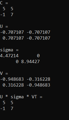
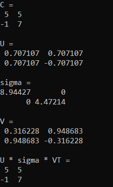
) sized MxN (it doesn’t have to be square) and breaks it apart into a rotation (U), a scale (\Sigma), and another rotation (V^T). Any matrix can be decomposed this way:
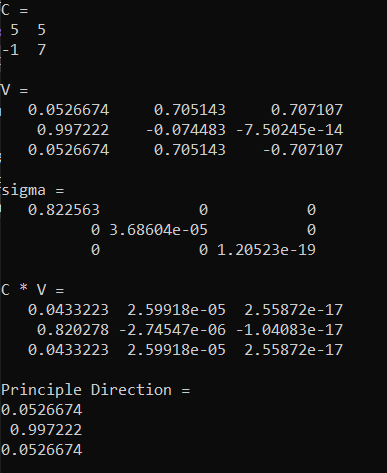
C = U \Sigma V^T

The scaling matrix \Sigma has zeros everywhere except the diagonal. The values on the diagonal are called the “Singular Values” and they also describe how “important” each row of U and column of V^T is. Just like PCA, you can get rid of the ones with the lowest singular values and thus reduce dimensionality of the data. This is called “Truncated SVD”.

So how do you calculate SVD?

First you multiply your (possibly rectangular) matrix C^T with C to make the square matrix C^TC.

The eigenvectors of C^TC get put together as column vectors to make the matrix V.

The matrix \Sigma has the square roots of the eigenvalues of C^TC along the diagonal.

The matrix U is made by multiplying C * V and normalizing the columns.

That’s all there is to it!

C++ Code

Using eigen to calculate SVD as described above is pretty straightforward:

Matrix2d C;
C <<
    5.0f, 5.0f,
    -1.0f, 7.0f;

// Calculate SVD as described in https://www.youtube.com/watch?v=cOUTpqlX-Xs
{
    Matrix2d CTC = C.transpose() * C;

    EigenSolver<Matrix2d> es(CTC);
    EigenSolver<Matrix2d>::EigenvalueType eigenValues = es.eigenvalues();
    EigenSolver<Matrix2d>::EigenvectorsType eigenVectors = es.eigenvectors();

    auto V = eigenVectors;

    MatrixXcd sigma;
    {
        sigma = MatrixXcd::Zero(eigenValues.rows(), eigenValues.rows());
        for (int i = 0; i < eigenValues.rows(); ++i)
            sigma(i, i) = sqrt(eigenValues[i].real());
    }

    MatrixXcd U = C * V;
    for (int i = 0; i < U.cols(); ++i)
        U.col(i).normalize();

    cout << "C = \n" << C << "\n\n";

    cout << "U = \n" << U.real() << "\n\n";
    cout << "sigma = \n" << sigma.real() << "\n\n";
    cout << "V = \n" << V.real() << "\n\n";

    cout << "U * sigma * VT = \n" << (U * sigma * V.transpose()).real() << "\n\n";
}

Running that gives this output. The final output of U*sigma*VT shows that putting the decomposed matrices back together gives you the original data.

While the Eigen library has interfaces to let you calculate eigenvalues and eigenvectors, it also has higher level functionality – including performing SVD itself! There are two ways to do SVD in Eigen… one is better for smaller matrices (JacobiSVD), the other is better for bigger matrices (BDCSVD). In this case, I use the one better for bigger matrices, because AFAIK it’s fine for smaller ones too, just a bit slower.

Matrix2d C;
C <<
	5.0f, 5.0f,
	-1.0f, 7.0f;

// Calculate SVD using the built in functionality
{
    BDCSVD<Matrix2d> svd(C, ComputeFullU | ComputeFullV);

    auto U = svd.matrixU();
    auto V = svd.matrixV();
    auto sigma = svd.singularValues().asDiagonal().toDenseMatrix();

    cout << "C = \n" << C << "\n\n";

    cout << "U = \n" << U << "\n\n";
    cout << "sigma = \n" << sigma << "\n\n";
    cout << "V = \n" << V << "\n\n";

    cout << "U * sigma * VT = \n" << U * sigma * V.transpose() << "\n\n";
}

Running that outputs this, which is the same as before, except the eigenvalues are switched, and one of the eigenvectors was multiplied by -1 (opposite magnitude but still the same eigenvector).

Calculating PCA With SVD

To calculate PCA using SVD, all you need to do is run SVD and then multiply C with V. Here’s some code where we use the 3×3 Gaussian kernel with sigma 0.3 from last blog post, and run PCA on it again.

// PCA!
{
    Matrix3d newC;
    newC <<
        0.002300, 0.043200, 0.002300,
        0.043200, 0.818000, 0.043200,
        0.002300, 0.043200, 0.002300;

    BDCSVD<Matrix3d> svd(newC, ComputeFullU | ComputeFullV);

    auto U = svd.matrixU();
    auto V = svd.matrixV();
    auto sigma = svd.singularValues().asDiagonal().toDenseMatrix();

    cout << "C = \n" << C << "\n\n";

    cout << "V = \n" << V << "\n\n";

    cout << "sigma = \n" << sigma << "\n\n";

    cout << "C * V = \n" << newC * V << "\n\n";

    cout << "Principle Direction = \n" << (newC * V).col(0).normalized() << "\n\n";
}

When we do that we get this. The sigma tells us that there is basically only one non zero component (the others are close enough to zero to be considered zero) and the principle direction matches what we found in the last post as well. Looks like it’s working!

SVD Of Image

Next up, we’ll take an image with size WxH, make a matrix that is Wx(3H) in size, and perform truncated SVD on it, with different numbers of singular values. The matrix is 3 times as tall because we are going to separate each row of RGB pixels into three rows of pixels; one row for each color channel. The code to do this is in the github repo, so go have a look and play around with it if you want to 🙂

First is the old man from legend of zelda 1 in NES. First is the original image, then 1 singular value, then 5%, 10%, 15%, 20%, 25% and 50%.

Next up is a different image, but the same percentages of singular values in the same order.

Using Truncated SVD In Practice

In the code I set singular values to zero to truncate SVD, but in reality if you wanted to truncate to N dimensions, you would shrink the sigma matrix to be NxN, and you would shrink the U and V matrix both to have N columns. In Eigen, you can do this using the “conservativeResize(rows, cols)” function.

Whether you have truncated or not, the U matrix can be considered your encoded data, and you can multiply sigma by V transpose to make the decoding matrix. Multiplying U by the decoding matrix will give you back your data, or an approximation to it if you truncated.

As a quick overview of what size of compressed data to expect, let’s say you have R rows of D dimensional data (an RxD matrix – R rows of data, and D columns of data).

When you SVD that, U will be RxR, Sigma will be RxR and V will be DxR. Multiplying sigma by V transpose to make the decoding matrix will be RxD. Multiplying U*Sigma*V transpose will be RxD.

Let’s say that you truncate the SVD data from being D dimensional to N dimensional. U will be RxN, Sigma will be NxN, and V will be DxN. Multiplying sigma by V transpose to make the decoding matrix will be NxD. Multiplying U*Sigma*V transpose will still be RxD.

When you have the U and sigma*V transpose matrices and you want to decode a single (scalar) value of data, you get the entire row from U that corresponds to your data’s R dimension, which will be M dimensional, and you get the entire column from the decoding matrix that corresponds to your data’s D dimension, which will also be M dimensional. You then dot product these vectors and have your decoded scalar value. This is useful if you want random access to your encoded data, such as in a shader on the GPU.

Knowing where to truncate to can be done by looking at the sigma values and finding where they taper off enough to your liking. Here is a graph of some SVD’d data where I divided all the singular values by the sum of the singular values to normalize them, and then I graphed the sum of the singular values at or before each dimension. You can see that this data is well fit by 3 or 4 dimensions.

The last 2 columns in this data show “Explained Variance” and “Culmulative Explained Variance” which is another metric to use to see how good a fit is for a certain number of dimensions. You calculate explained variance by dividing sigma squared by the sum of all sigmas squared. For culmulative explained variance, you sum up the sigmas squared at or before the dimension you are looking at, divided by the sum of all sigmas squared.

An intuitive perspective to SVD for data compression is that if you have some data that is AxB in size, SVD will break it into three matrices: an AxA matrix, an AxA scaling matrix, and an AxB matrix. You can multiply the middle scaling matrix into either the left or the right matrix and then end up with only two matrices: one is AxA and the other is AxB. At this point, our data is larger than it used to be, but that scaling matrix told us how important each column of the first matrix / row of the second matrix is. We can remove those for any place that the scaling matrix is zero or close enough to zero to be considered zero. That gives us two matrices AxN and NxB. At this point, if (A*N + N*B) is smaller than (A*B) then we’ve compressed our data in a nearly lossless way.

We don’t have to stop here though, and can start trimming more rows and columns off to make the matrices be AxM and MxB, such that (A*M + M*B) is smaller than (A*B) by as much as we want – but we introduce error into the process and our compression is no longer lossless. The error we are adding is minimized in the “least squares” sense, so it will be many small errors instead of a few large errors, which is often desired in practice.

A matrix multiply is all that is needed to get your data back, but individual values can be read back easily as well (random access). You get the a’th row from the first matrix, and the b’th column from the second matrix. The vectors will both be of size M. You dot product them, and your value is “decompressed”.

If doing something like compressing animation, the first matrix might be indexed by time, and the second matrix might be indexed by bone id*3, having 3 entries for the position of a bone starting at that bone id*3 location in the matrix. Then it’s just a vec3 * mat3x3 multiply (or alternately 3 dot products) to get the position back.

Shorter Intuition & Practical Concerns (Added 10/2/22)

Here is some shorter intuition for using truncated SVD for data compression.

If you start with data that is W * H in size, this lets you make it into data that is (W + H) * N in size, where N is tuneable for quality vs size. The U matrix will be W * N in size, and the SigmaV matrix will be H * N in size.

To decompress a single value at (X,Y), you read an N sized vector from U, an N sized vector from SigmaV, and dot product them to get the value back.

The downside to this technique is the memory (texture) reads, where for each value you want to decompress you need to read 2*N values to dot product them together.

Closing And Links

The Eigen library is pretty neat. You can grab the latest zip from https://eigen.tuxfamily.org/ and after unzipping, the “Eigen” folder within the zip has the files you want to include in your program.

Compilation times are pretty long when including files from this library, which i found surprising. It’d probably be best to put the includes to Eigen within a static library that didn’t get changed often to avoid the compilation times. I also had to turn on \bigobj in msvc after hitting an error regarding it.

Other than that, I’m a fan of Eigen and expect to use it when I need to do things like this, instead of writing from scratch, or calling into python scripts to do these numerical operations (hehe).

Here is a great use of SVD to compress PBR textures:
https://bartwronski.com/2020/05/21/dimensionality-reduction-for-image-and-texture-set-compression/

Here are some links I found useful when learning SVD:
https://jonathan-hui.medium.com/machine-learning-singular-value-decomposition-svd-principal-component-analysis-pca-1d45e885e491 
https://youtu.be/DG7YTlGnCEo
https://youtu.be/Jqg7JgCwQrk
https://towardsdatascience.com/simple-svd-algorithms-13291ad2eef2 
https://medium.com/swlh/truncated-singular-value-decomposition-svd-using-amazon-food-reviews-891d97af5d8d

Programming PCA From Scratch In C++

When running PCA (Principle Component Analysis) on a data set, it gives back a set of orthogonal axes for that data, as well scalar values telling you the importance of each axis.

When sorting the axes by importance, the first axis is the axis that has the most variation of the data, so is the best approximation of the data with a straight line. The second axis is perpendicular and is the axis that adds the most variation of the error from the first line. The third axis is perpendicular and adds on the most remaining variation, same with the fourth, fifth and so on, up to the dimensionality of your data set.

While you can transform your data to use these axes and reconstruct the data perfectly, PCA is useful because you can decide to throw away some number of the least important axes, thus reducing the dimensionality of the data!

That can be useful for data analysis (reasoning about 2D data is a lot easier than 4D data!), but it can also be a form of data compression, if the error introduced by throwing away one or more dimensions is acceptable.

PCA itself is pretty easy to explain, but to implement it yourself, you need to be able to calculate the eigen values and eigen vectors of a matrix. Those operations are notoriously difficult to do in robust ways, so the common wisdom is to not implement them yourself, but to use software like python or libraries like Eigen (https://eigen.tuxfamily.org/) to do the hard bits for you.

To crack open the black box a bit though, I implemented it in plain C++. It’s about 800 lines including comments, generated all the data in this blog post, and you can check it out here: https://github.com/Atrix256/PCA.

Calculating PCA

To calculate PCA you…

  1. Center the data
  2. Calculate the covariance matrix
  3. Calculate the covariance eigen values and eigen vectors
  4. Transform the data
  5. Recover the data

Let’s go through this step by step.

1. Center the Data

For this you just calculate the average of your data and subtract the average from all data points.

This makes the data centered on the origin which is important for PCA since it is meant to find the axes of importance in the data – NOT fit a line to the data.

Later on if you want to recover your uncentered data from the PCA encoded data, you’ll need to keep this average around to add it back in. Something to keep in mind if thinking about using PCA for data compression.

2. Calculate the Covariance Matrix

If you have N dimensional data, the covariance matrix will be NxN.

Each cell of the covariance matrix i,j will contain the covariance value between all the data in dimension i and dimension j. Since the covariance of a variable with itself is the variance, the diagonal of the matrix will have the variance values of the dimensions.

As a recap, covariance is calculated as:

cov(X,Y) = \mathbb{E}(XY) - \mathbb{E}(X) * \mathbb{E}(Y)

Variance is just covariance of a value with itself, so is calculated as:

var(X) = \mathbb{E}(X^2) - \mathbb{E}(X)^2

If your data represents a sample of the data instead of the entire data, you’ll need to use sample variance instead, which divides the sums by (n-1) instead of dividing by n.

3. Calculate the Covariance Eigen Values and Eigen Vectors

This is the part that is less easy, where we calculate the eigen values and eigen vectors of the covariance matrix. The eigen vectors are the axes of importance we mentioned before, and the eigen values are how important each one is.

First we need to calculate the eigen values.

I calculate them using the “QR Algorithm” (https://en.wikipedia.org/wiki/QR_algorithm) which is an algorithm that gives you approximate eigen values. It works by repeatedly doing QR decomposition (https://en.wikipedia.org/wiki/QR_decomposition) on the matrix and setting the matrix to R*Q for the next iteration. You do this process until a certain number of iterations has occurred, or all non diagonal elements of the matrix are close enough to zero for your liking. When finished, the approximate eigen values are the diagonal values of the matrix.

I loop until the largest non diagonal value is less than 0.0001, but didn’t play around with this very much. You can see this code at https://github.com/Atrix256/PCA/blob/main/vecmath.h#L321.

As part of the QR decomposition, I use the Gram-Schmidt process (https://en.wikipedia.org/wiki/Gram%E2%80%93Schmidt_process) to make orthogonal vectors.

There are other ways to get eigen values, and other choices you can make in the QR algorithm. I didn’t implement shifting, which helps convergence, and I’ve heard that Householder reflections are much better quality, and not that much more difficult to implement.

In any case, this works well enough for me to get good enough eigen values in my test cases.

Now that we have the eigen values, we need to get the eigen vector associated with each one. To do that, I use the inverse iteration algorithm (https://en.wikipedia.org/wiki/Inverse_iteration) which gives you an eigenvector associated with an approximate eigen value. It’s a pretty simple algorithm that just inverts a matrix and then repeatedly puts a randomly initialized vector through it. I do that for 10,000 iterations. The code for it is at https://github.com/Atrix256/PCA/blob/main/vecmath.h#L398.

I also normalize the eigen vectors and re-calculate the eigen values from the newly found eigen vectors to make them match up better. I had to switch from floats to doubles at one point as well, but may have just been doing something silly, like letting numbers get too small without clamping them to zero.

4. Transform the data

Sorting the eigen vectors from largest to smallest, you can then make them be columns of a matrix. This is the matrix you use to convert your data into “PCA space”. To reduce dimensionality you can either throw away columns from the right at this point, or you can wait until after transforming the data into the new space. It’s up to you to decide how many columns you can get away with throwing away for your usage case.

5. Recover the Data

To recover your data from “PCA space”, you make the eigenvectors for the dimensions that you didn’t throw out as rows in a matrix instead of columns. Multiply the PCA data by this matrix to get the data back minus the information contained in the lost columns.

Not too bad right? I want to re-iterate that while this code works for my handful of test cases on this blog post, it almost certainly is not production ready. It’s just a semi naive implementation for learning purposes.

Result: Gaussian Blur Kernel

First let’s PCA a 3×3 gaussian blur kernel with a sigma of 0.3.

The filter itself is:

[0.002300, 0.043200, 0.002300]
[0.043200, 0.818000, 0.043200]
[0.002300, 0.043200, 0.002300]

The eigen values and eigen vectors are:

[0.134147] [0.052641, 0.997225, 0.052641]
[0.000000] [0.000000, 0.000000, 0.000000]
[0.000000] [0.000000, 0.000000, 0.000000]

Interestingly, you can see that there’s only one non zero eigenvalue. That means that our data is in fact a rank 1 matrix in disguise! In other words, all the rows are just scalar multiples of each other. We could then replace each row with a single scalar value to multiply the eigen vector by which would reduce our data from 3D to 1D and 1/3 the storage size!

The two rows of zero eigen values is due to the fact that gaussian blurs are separable, so rows (or columns) really are just scalar multiples of each other. This test was inspired by a post from Bart Wronski on how to use SVD to separate non separable filters: https://bartwronski.com/2020/02/03/separate-your-filters-svd-and-low-rank-approximation-of-image-filters/

Result: 2D Data

Here’s the eigenvectors of some 2D data, then showing it reduced to 1 dimension along the larger eigenvector, then showing it including the smaller eigenvector, which makes it fit the data perfectly.

Here is the same with some different data points.

Result: 3D Data

I took some 3D data from a page that was real helpful when trying to understand PCA better (https://towardsdatascience.com/the-mathematics-behind-principal-component-analysis-fff2d7f4b643):

[90.000000, 60.000000, 90.000000]
[90.000000, 90.000000, 30.000000]
[60.000000, 60.000000, 60.000000]
[60.000000, 60.000000, 90.000000]
[30.000000, 30.000000, 30.000000]

The eigen values and eigen vectors are:

[910.069953] [0.655802, 0.429198, 0.621058]
[629.110387] [0.385999, 0.516366, -0.764441]
[44.819660] [0.648790, -0.741050, -0.172964]

And here is the RMSE for the data when PCA’d to different numbers of dimensions:

[1] 25.960163
[2] 6.694749
[3] 0.000000

At 1 component the data is:

[88.540569, 74.751951, 81.346364]
[72.547174, 64.284878, 66.200303]
[63.419540, 58.311187, 57.556254]
[75.638271, 66.307884, 69.127633]
[29.854445, 36.344100, 25.769445]

At 2 components:

[83.264247, 67.693599, 91.795721]
[90.954764, 88.909466, 29.745464]
[62.525570, 57.115286, 59.326695]
[65.892097, 53.270028, 88.429194]
[27.363322, 33.011622, 30.702926]

At 3 components, it matches, since no dimensionality reduction occured.

[90.000000, 60.000000, 90.000000]
[90.000000, 90.000000, 30.000000]
[60.000000, 60.000000, 60.000000]
[60.000000, 60.000000, 90.000000]
[30.000000, 30.000000, 30.000000]

Closing and Links

When you fit PCA to data, it minimizes the distance from the data point to the fit line. This is in contrast to least squares which only minimizes the distance on the y axis. One reason I wanted to dive deep into PCA was to see if it could be used to fit piecewise non linear curves like least squares can. After learning more, that seems to be swimming against the current for PCA, which is more aimed at things like making 3d vectors be storable as 2d vectors. I’ll bet what I was thinking of is possible, but I couldn’t really find info on it. I did find out that “Total Least Squares” exists which does the same kind of fitting though, so I think I should look more into that. Also “non linear dimensional reduction” is a topic as well.

It turns out too that a better way to do PCA than what I’ve done above is to use SVD to do PCA. I plan on doing a post on SVD soon and should be able to talk more about that then.

These two links were super helpful while writing this code:
https://towardsdatascience.com/the-mathematics-behind-principal-component-analysis-fff2d7f4b643
https://towardsdatascience.com/principal-component-analysis-explained-d404c34d76e7

Since rolling your own PCA is usually frowned on due to the numerical complexity of things involved, here’s some info about how to do PCA in python (also, in C++ you might want to use that Eigen library i mentioned before)
https://stats.stackexchange.com/questions/235882/pca-in-numpy-and-sklearn-produces-different-results

Check out this link for a neat usage case of PCA for texture compression on textures used in PBR (Physically Based Rendering):
https://bartwronski.com/2020/05/21/dimensionality-reduction-for-image-and-texture-set-compression/