The last post talked about links between Euler’s number e, and probability, inspired by a really cool youtube video on the subject: https://www.youtube.com/watch?v=AAir4vcxRPU
One of the things illustrated is that if you want to evaluate N candidates and pick the best one, you can evaluate the first N/e candidates (~36.8%), keep track of the highest score, then start evaluating the rest of the candidates, and choose the first one that scores higher.
That made me think of “Mitchell’s Best Candidate” algorithm for generating blue noise sample points. It isn’t the most modern way to make blue noise points, but it is easy to describe, easy to code, and gives decent-quality blue noise points.
If you already have N blue noise points (N can be 0)
Generate N+1 white noise points as candidates.
The score for a candidate is the distance between it and the closest existing blue noise point.
Keep whichever candidate has the largest score.
The above generates one more blue noise point than you have. You repeat that until you have as many points as you want.
So, can we merge these two things? The idea is that instead of generating and evaluating all N+1 candidates, we generate and evaluate (N+1)/e of them, keeping track of the best score.
We then generate more candidates, until we find a candidate with a better score, and then exit, or until we run out of candidates, at which case we return the best candidate we found in the first (N+1)/e of them.
This is done through a simple modification in Mitchell’s Best Candidate algorithm:
We calculate a “minimum stopping index” which is ceil((N+1)/e).
When we are evaluating candidates, if we have a new best candidate, and the candidate index is >= the minimum stopping index, we exit the loop and stop generating and evaluating candidates.
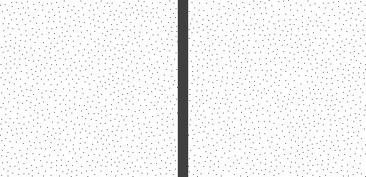
Did it work? Here are two blue noise sets side by side. 1000 points each. Can you tell which is which?
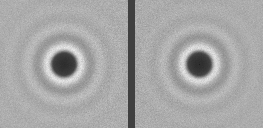
Here are the averaged DFTs of 100 tests.
In both sets of images, the left is Mitchell’s Best Candidate, and the right is Euler’s Best Candidate.
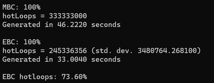
The program output shows us that EBC took 71% of the time that MBC did though. Also, the inner most loop of these best candidate algorithms is calculating the distance between a candidate and an existing point. EBC only had to do 73.6% of these calculations as MBC did for the same quality result. While MBC has a fixed number of “hot loops”, EBC is randomized though and has a standard deviation of 3.5 million, when the operation takes at max 333 million, so has a standard deviation of about 1%.
It looks like a win to me! Note that the timing includes writing the noise to disk as pngs.
This could perhaps be a decent way to do randomized organic object placement on a map, like for bushes and trees and such. There are other algorithms that generate several candidates and keep the best one though. It should work just fine in those situations as well. Here is a mastodon thread on the subject https://mastodon.gamedev.place/@demofox/110030932447201035.
The next time you have to evaluate a bunch of random candidates to find the best one, you can remember “find the best out of the first 1/3, then continue processing til the next best one you find, or you run out of items”.
For more info, check out this Wikipedia page, which also talks about variations such as what to do if you don’t know how many candidates you are going to need: https://en.wikipedia.org/wiki/Secretary_problem
It was a lot of the same old stuff we’ve all seen many times before but then started talking about Euler’s number showing up in probability. The video instantly had my full attention.
I spend a lot of time thinking about how uses of white noise can be turned into using blue noise or low discrepancy sequences because white noise has nice properties at the limit, but those other things have the same properties over much smaller numbers of samples. This link to probability made we wonder how other types of noise / sequences would behave when put through the same situations where Euler’s number emerged. Would e still emerge, or would it be a different value for different sequence types?
This is what sent me on the rabbit hole for the two prior blog posts, which explore making streaming uniform red noise, blue noise, and other random number generators.
Let’s get into it!
Lottery Winnings
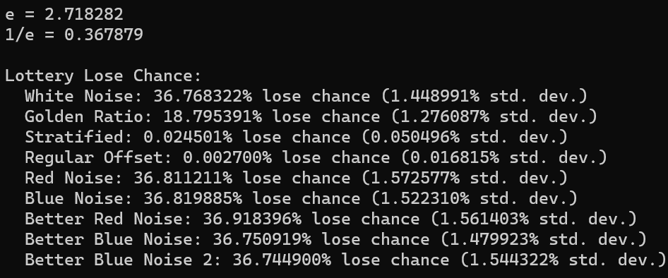
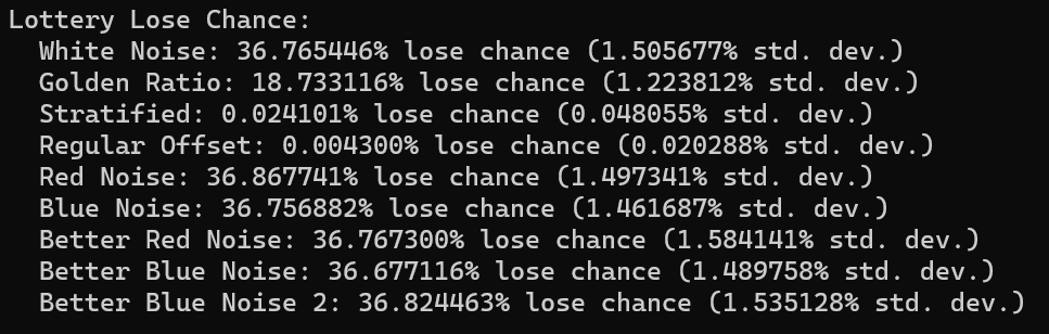
One claim the video makes is that if the odds for winning the lottery are 1 in N, that if you buy N lottery tickets, there is a 1/e chance that you will still lose. 1/e is 0.367879, so that is a 36.79% of losing.
That may be true for white noise, but how about other sequences?
To test, I generate a random integer in [0,N) as the winning number, and then generate N more random numbers as the lottery tickets, each also in [0, N). The test results in a win (1) or a loss (0). This test is done 1,000,000 times to get an average chance of losing. Also, standard deviation is calculated by looking at the percentage of each group of 1,000 tests.
Here are the sequences tested:
White Noise – regular old random numbers
Golden Ratio – the deterministic golden ratio sequence: fract(index * phi)
Stratified – stratify N buckets to make N numbers
Regular Offset – N regularly spaced numbers, but with a random offset and modulus to keep them in range.
Blue Noise – made by subtracting one value from another, converting from triangle to uniform, and rerolling one of the numbers for next time. Each number gets regenerated every other index, and which value gets subtracted changes each index as well. (https://blog.demofox.org/2023/02/20/uniform-1d-red-noise-blue-noise/)
We were able to duplicate the results for white noise which is neat. Using the golden ratio sequence cuts the loss rate in half. I chalk this up to it being more fairly distributed than white noise. White noise is going to give you the same lottery ticket number several times, where golden ratio is going to reduce that redundancy.
Stratified and regular offset both did very well on this test, but that isn’t surprising. If you have a 1 in N chance of picking a winning random number, and you make (almost) every number between 1 and N as a guess, you are going to (almost) always win. The little bit of randomization in each will keep them from winning 100% of the time.
the red noise and blue noise were very close to having a 1/e loss chance but were off in the tenths of a percentage place. Running it again gives similar results, so I think this could be a real, but small, effect. Colored noise seems like it affects this outcome a little bit.
Summing Random Values
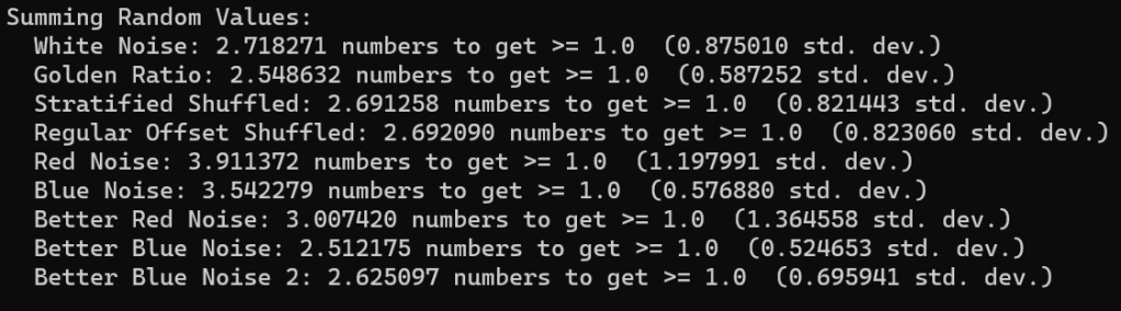
Another claim the video makes is that if you add random uniform white noise numbers together, it will on average take e of them (2.718282) to be greater than or equal to 1. I do that test 100,000,000 times with each sequence again.
Let’s see:
We duplicated the results with white noise again, which is neat.
The golden ratio sequence takes slightly fewer numbers to reach 1.0. Subsequent numbers of the golden ratio sequence are pretty different usually, so this makes some sense to me.
For stratified and regular offset, I wanted to include them, but their sequence is in order, which doesn’t make sense for this test. So, I shuffled them. The result looks to be just a little bit lower than e.
The lower quality red and blue noise took quite a bit more numbers to reach 1.0 at 3.9 and 3.5 respectively. The better red noise took 3 numbers on average, while the blue noise took the lowest seen at 2.5 numbers. Lastly, the FIR blue noise “better blue noise 2” took just under e.
An interesting observation is that the red noises all have higher standard deviation than the other sequences. Red noise makes similar numbers consecutively, so if the numbers are smaller, it would take more of them, where if they were bigger it would take fewer of them. I think that is why the standard deviation (square root of variance) is higher. It’s just more erratic.
Contrary to that, the blue noise sequences have lower standard deviation. Blue noise makes dis-similar numbers consecutively, so I think it makes sense that it would be more consistent in how many numbers it took to sum to 1.0, and thus have a lower standard deviation and variance.
Finding The Best Scoring Item
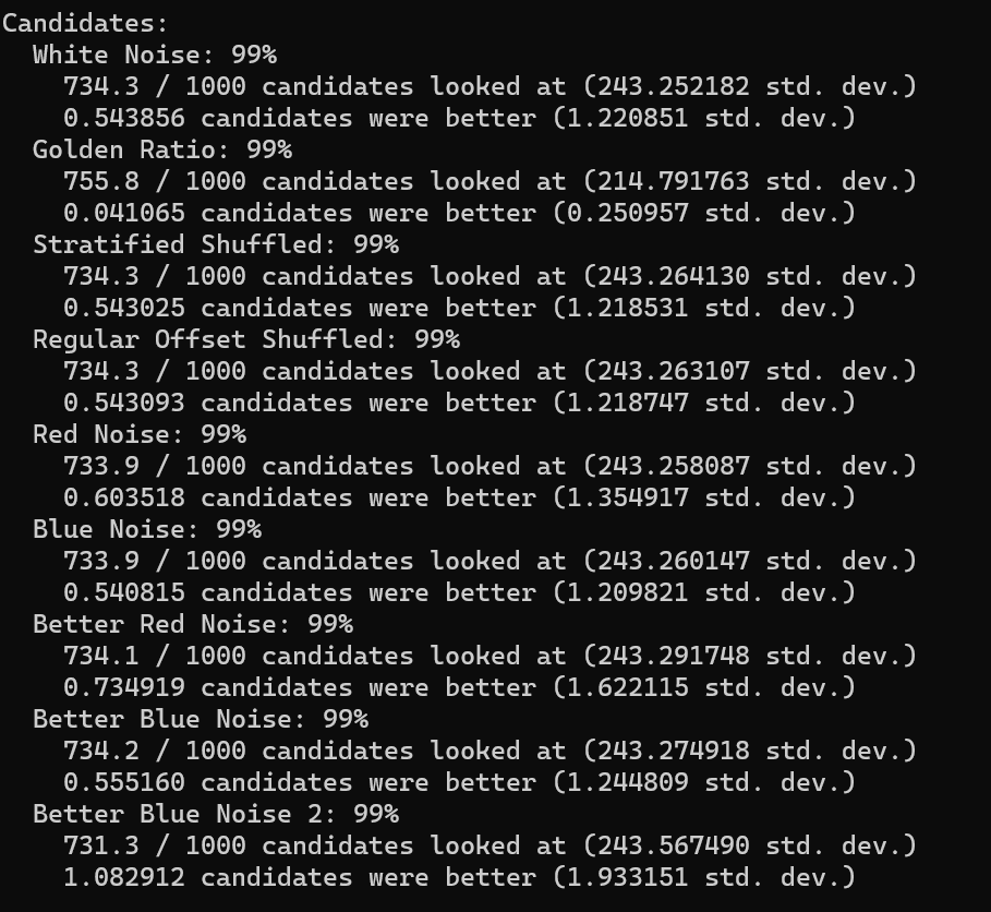
The video also had this neat algorithm for fairly reliably finding the best scoring item, without having to look at all items.
Their setup is that you have job applicants to review and after talking to each, you have to decide right then to hire the person or to continue looking at other candidates. The algorithm is that you interview 1/e percent of them (36.79%), not hiring any of them, but keeping track of how well the best interviewer did. You then start interviewing the remaining candidates and hire the first one that does better than the previous best.
Doing this apparently gives you a 1/e (36.79%) chance of picking the actual best candidate, even though you don’t evaluate all the candidates. That is pretty neat.
I did this test 10,000,000 times for each sequence type
All sequence types looked at 733 or 734 candidates out of 1000 on average. The golden ratio sequence actually ended up looking at 755 on average though, and the better blue noise 2 sequence looked at 731. The standard deviation is ~243 for all of them, except for golden ratio which is 214. So… golden ratio looks at more candidates on average, but it’s also more consistent about the number of candidates it looks at.
Most sequence types had roughly 0.5 candidates on average better than the candidate hired. The golden ratio has 0.04 candidates better on average though. Red noise has slightly more candidates better than that though, at 0.6 and 0.73. The “Better Blue Noise 2” has a full 1.08 candidates better on average. The standard deviation follows these counts… golden ratio is the lowest standard deviation by far, red noise is higher than average, and the better blue noise 2 is much higher than the rest.
Closing
As usual, the lesson is that DSP, stochastic algorithms and sampling are deep topics.
My last blog post was on filtering a stream of uniform white noise to make a stream of red or blue noise, and then using the CDF (inverted inverse CDF) to transform the non uniform red or blue noise back into a uniform distribution while preserving the noise color. It is at https://blog.demofox.org/2023/02/20/uniform-1d-red-noise-blue-noise/
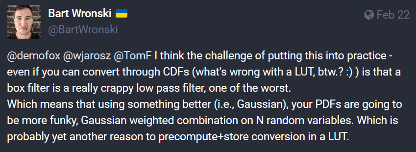
That had me thinking about how you could make a CDF of any distribution, numerically. You could then store it in a LUT, or perhaps use least squares to fit a polynomial to the CDF.
I had never seen that before, only ever seeing that you can subtract a low pass filter from the identity filter to get a high pass filter (https://blog.demofox.org/2022/02/26/image-sharpening-convolution-kernels/). It made me want to check out that kind of a filter to see what the differences could be.
So, I started by generating 10 million values of white noise and then filtering it. I made a histogram of the results and divided the counts by 10 million to normalize it into a PDF. From there I made a CDF by making a table where each CDF bucket value was the sum of all PDF values with the same or lower index. From there I made a 1024 entry CDF table, as well as a smaller 64 entry one, and I also fit the CDF with piecewise polynomials (https://blog.demofox.org/2022/06/29/piecewise-least-squares-curve-fitting/).
With any of those 3 CDF approximations, I could filter white noise in the same way I did when generating the CDF, put the colored noise through the CDF function, and get out colored noise that was uniform distribution.
I wasn’t very happy with the results though. They were decent, but I felt like I was leaving some quality on the table. Going from real values to indices and back was a bit fiddly, even when getting the nuances correct. I mentioned that it was surprisingly hard to make a usable CDF from a histogram, and Nikita gave this great comment.
The intuition here is that regions of values that are more probable will take up more indices and so if you randomly select an index, you are more likely to select from those regions.
So, if you have a black box that is giving you random numbers, you can generate random numbers from the same distribution just by storing a bunch of the numbers it gives you, sorting them, and using uniform random numbers to select items from that list. Better yet, select a random position between 0 and 1, multiply by the size of the list, and use linear interpolation between the indices when you get a fractional index.
In our case where we are trying to make non uniform numbers be uniform again, we actually want the inverted inverse CDF, or in other words, we want the CDF. We can get a CDF value from the inverse CDF table by taking a value between 0 and 1 and finding where it occurs in the inverse CDF table. We’ll get a fractional index out if we use linear interpolation, and we can divide by the size of the array to get a value between 0 and 1. This is the CDF value for that input value. If we do this lookup for N evenly spaced values between 0 and 1, we can get a CDF look up table out.
I did that with a 1024 sized look up table, a 64 sized look up table, and I also fit a piecewise polynomial to the CDF, with piecewise least squares.
The results were improved! Fewer moving parts and fewer conversions. Nice.
I’ll show the results in a minute but here are the tests I did:
Box 3 Red Noise: convolved the white noise with the kernel [1, 1, 1]
Box 3 Blue Noise: convolved the white noise with the kernel [-1, 1, -1]. This is an unsharp mask because I subtracted the red noise kernel from [0,2,0].
Box 5 Red Noise: [1,1,1,1,1]
Box 5 Blue Noise 1: [-1, -1, 1, -1, -1]
Box 5 Blue Noise 2: [1, -1, 1, -1, 1]
Gauss 1.0 Blue Noise: A sigma 1 gaussian kernel, with alternating signs to make it a high pass filter [0.0002, -0.0060, 0.0606, -0.2417, 0.3829, -0.2417, 0.0606, -0.0060, 0.0002]. Kernel calculated from here http://demofox.org/gauss.html
FIRHPF – a finite impulse response high pass filter. It’s just convolved with the kernel [0.5, -1.0, 0.5]. Kernel calculated from here http://demofox.org/DSPFIR/FIR.html/
IIRHPF – an infinite impulse response high pass filter. It has the same “x coefficients” as the previous filter, but has a y coefficient of 0.9. Filter calculated from here http://demofox.org/DSPIIR/IIR.html.
FIRLPF – the low pass filter version of FIRHPF. kernel [0.25, 0.5, 0.25]
IIRLPF – the low pass filter version of IIRHPF. x coefficients are the same as the previous filter, but has a y coefficient of -0.9.
Void And Cluster – I used the void and cluster algorithm to make 100,000 blue noise values, and I did this 100 times to get 10 million total blue noise values. There is a “seam” in the blue noise every 100,000 values but that shouldn’t be a big deal.
Final BN LUT – I took the sized 64 CDF LUT from the FIRHPF test and used it to turn filtered white noise back to uniform.
Final BN Polynomial – I took the 4 piecewise quadratic functions that fit the CDF of FIRHPF and used it to turn filtered white noise back to uniform.
Final RN Polynomial – The filter from FIRLPF is used, along with the polynomial from the previous filter to make it uniform again. Luckily FIRLPF and IIRLPF have the same histogram and CDF, so can use the same polynomials!
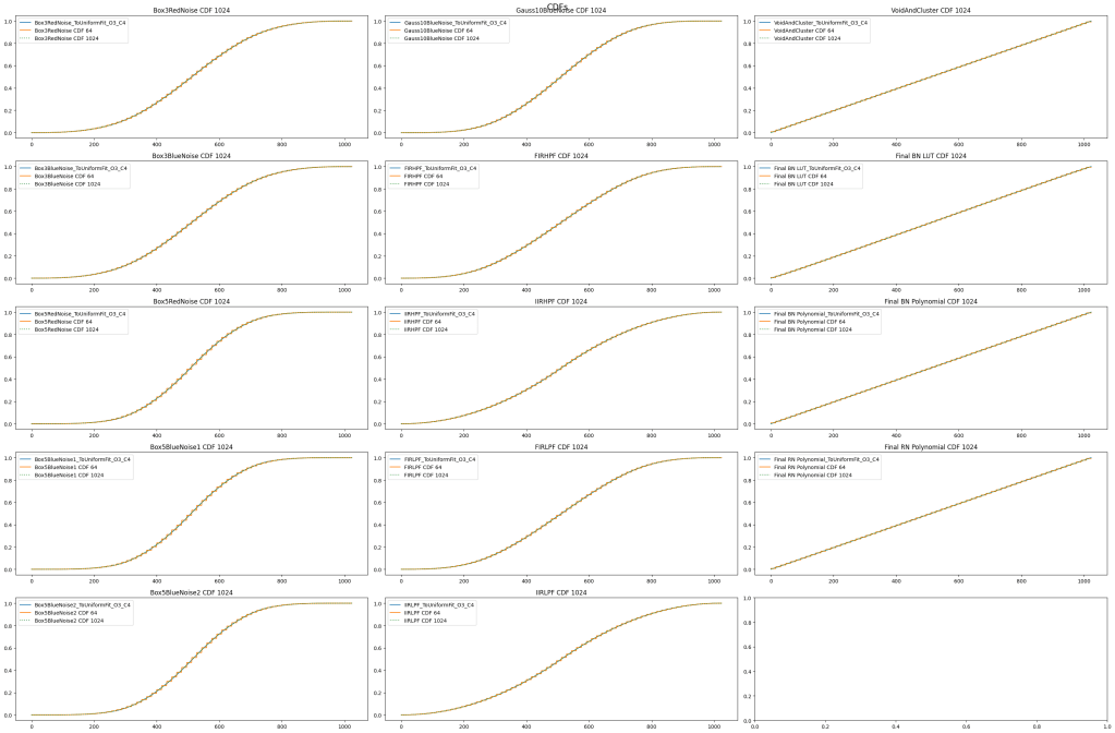
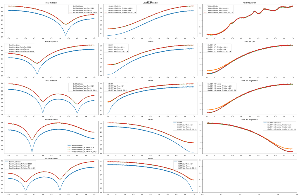
CDFs
In the below, the blue line is the 4 piecewise quadratic functions fit to the CDF. The green dotted line is the size 1024 CDF table. The orange line is the size 64 CDF table.
For void and cluster, and the “Final BN” tests, the source values are uniform, so it doesn’t make much sense to make a CDF and convert them to uniform etc, but it wasn’t trivial to disable that testing for them.
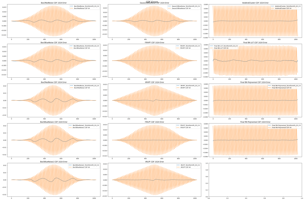
Here is the error of the CDF approximations, using the size 1024 CDF LUT as the ground truth to calculate the error.
Frequencies (DFTs)
Here are the DFTs to show the frequencies in the streams of noise. Converting filtered white noise to uniform does change the frequency a bit, but looking at the low frequency magnitudes of void and cluster, that might just be part of the nature of uniform distributed colored noise. I’m not sure.
The blue line is the original values from E.g. filtering white noise. The other colors are when converting them to uniform.
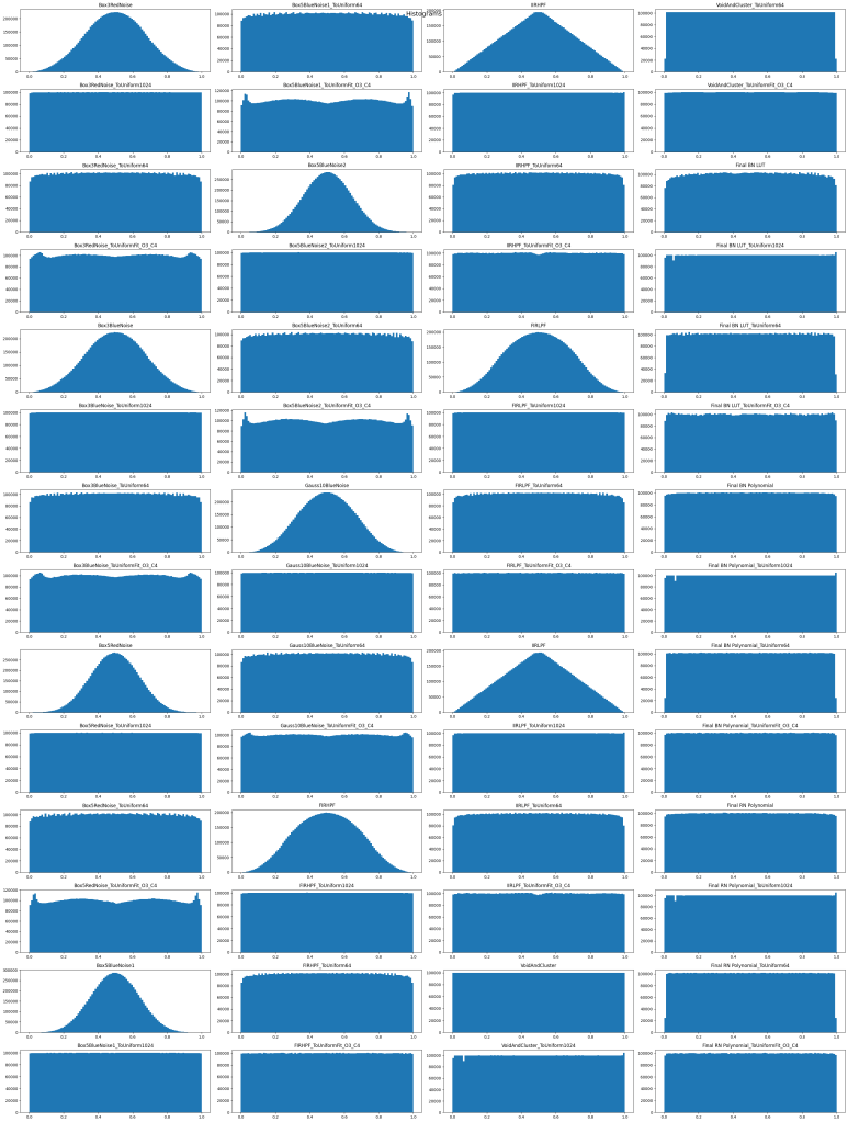
Histograms
Here are the histograms, to see if they are appropriately uniform. The histograms come in sets of 4: the filtered noise, and then 3 methods for converting the filtered noise back to uniform. The graphs should be red from top to bottom, then left to right.
Streaming Blue Noise
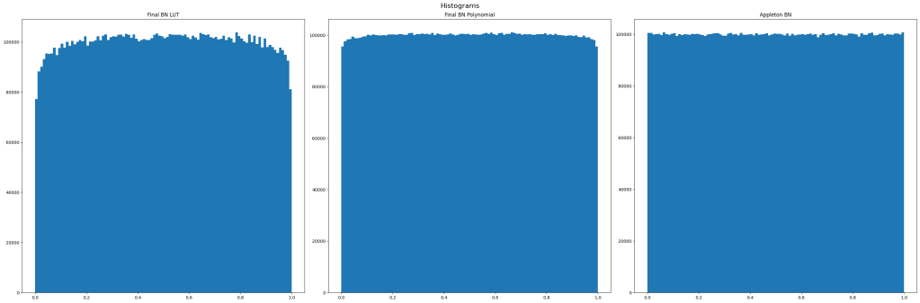
Looking at the results, the FIRHPF results look pretty decent, with the polynomial fit having a better histogram than the size 64 CDF LUT. Only being a 3 tap filter means that it only needs to remember the last 2 “x values” that it has seen too, as a “delay line” for the FIR filter. Decent quality results and efficient to obtain. nice. The results of that are in the diagrams above as “Final BN Polynomial”.
I tried taking only the first half of the fits – either 32 of the 64 LUT entries, or only the first two of the four polynomials. For the second half of the curve, when x > 0.5, you set x to1-x, and the resulting y value gets flipped as 1-y too. I wasn’t getting great results though, even when adding a least squares constraint that CDF(0.5) = 0.5. I’m saving that battle for a future day. If you solve it though, leave a comment!
Below is the C++ code for streaming scalar valued blue noise – aka a blue noise PRNG. Also the same for red noise. The full source code can be found at https://github.com/Atrix256/ToUniform.
If you have a need of other colors of noise, of other histograms, hopefully, this post can help you achieve that.
class BlueNoiseStreamPolynomial
{
public:
	BlueNoiseStreamPolynomial(pcg32_random_t rng)
		: m_rng(rng)
	{
		m_lastValues[0] = RandomFloat01();
		m_lastValues[1] = RandomFloat01();
	}

	float Next()
	{
		// Filter uniform white noise to remove low frequencies and make it blue.
		// A side effect is the noise becomes non uniform.
		static const float xCoefficients[3] = {0.5f, -1.0f, 0.5f};

		float value = RandomFloat01();

		float y =
			value * xCoefficients[0] +
			m_lastValues[0] * xCoefficients[1] +
			m_lastValues[1] * xCoefficients[2];

		m_lastValues[1] = m_lastValues[0];
		m_lastValues[0] = value;

		// the noise is also [-1,1] now, normalize to [0,1]
		float x = y * 0.5f + 0.5f;

		// Make the noise uniform again by putting it through a piecewise cubic polynomial approximation of the CDF
		// Switched to Horner's method polynomials, and a polynomial array to avoid branching, per Marc Reynolds. Thanks!
		float polynomialCoefficients[16] = {
			5.25964f, 0.039474f, 0.000708779f, 0.0f,
			-5.20987f, 7.82905f, -1.93105f, 0.159677f,
			-5.22644f, 7.8272f, -1.91677f, 0.15507f,
			5.23882f, -15.761f, 15.8054f, -4.28323f
		};
		int first = std::min(int(x * 4.0f), 3) * 4;
		return polynomialCoefficients[first + 3] + x * (polynomialCoefficients[first + 2] + x * (polynomialCoefficients[first + 1] + x * polynomialCoefficients[first + 0]));
	}

private:
	float RandomFloat01()
	{
		// return a uniform white noise random float between 0 and 1.
		// Can use whatever RNG you want, such as std::mt19937.
		return ldexpf((float)pcg32_random_r(&m_rng), -32);
	}

	pcg32_random_t m_rng;
	float m_lastValues[2] = {};
};

class RedNoiseStreamPolynomial
{
public:
	RedNoiseStreamPolynomial(pcg32_random_t rng)
		: m_rng(rng)
	{
		m_lastValues[0] = RandomFloat01();
		m_lastValues[1] = RandomFloat01();
	}

	float Next()
	{
		// Filter uniform white noise to remove high frequencies and make it red.
		// A side effect is the noise becomes non uniform.
		static const float xCoefficients[3] = { 0.25f, 0.5f, 0.25f };

		float value = RandomFloat01();

		float y =
			value * xCoefficients[0] +
			m_lastValues[0] * xCoefficients[1] +
			m_lastValues[1] * xCoefficients[2];

		m_lastValues[1] = m_lastValues[0];
		m_lastValues[0] = value;

		float x = y;

		// Make the noise uniform again by putting it through a piecewise cubic polynomial approximation of the CDF
		// Switched to Horner's method polynomials, and a polynomial array to avoid branching, per Marc Reynolds. Thanks!
		float polynomialCoefficients[16] = {
			5.25964f, 0.039474f, 0.000708779f, 0.0f,
			-5.20987f, 7.82905f, -1.93105f, 0.159677f,
			-5.22644f, 7.8272f, -1.91677f, 0.15507f,
			5.23882f, -15.761f, 15.8054f, -4.28323f
		};
		int first = std::min(int(x * 4.0f), 3) * 4;
		return polynomialCoefficients[first + 3] + x * (polynomialCoefficients[first + 2] + x * (polynomialCoefficients[first + 1] + x * polynomialCoefficients[first + 0]));
	}

private:
	float RandomFloat01()
	{
		// return a uniform white noise random float between 0 and 1.
		// Can use whatever RNG you want, such as std::mt19937.
		return ldexpf((float)pcg32_random_r(&m_rng), -32);
	}

	pcg32_random_t m_rng;
	float m_lastValues[2] = {};
};
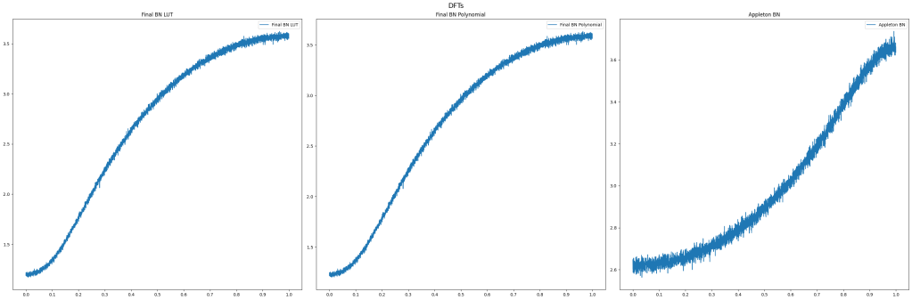
I coded it up and put it through my analysis so you could compare apples to apples. It looks pretty good!
Histograms
DFTs
Code
// From Nick Appleton:
// https://mastodon.gamedev.place/@nickappleton/110009300197779505
// But I'm using this for the single bit random value needed per number:
// https://blog.demofox.org/2013/07/07/a-super-tiny-random-number-generator/
// Which comes from:
// http://www.woodmann.com/forum/showthread.php?3100-super-tiny-PRNG
class BlueNoiseStreamAppleton
{
public:
	BlueNoiseStreamAppleton(unsigned int seed)
		: m_seed(seed)
		, m_p(0.0f)
	{
	}

	float Next()
	{
		float ret = (GenerateRandomBit() ? 1.0f : -1.0f) / 2.0f - m_p;
		m_p = ret / 2.0f;
		return ret;
	}

private:
	bool GenerateRandomBit()
	{
		m_seed += (m_seed * m_seed) | 5;
		return (m_seed & 0x80000000) != 0;
	}

	unsigned int m_seed;
	float m_p;
};