
The simple standalone C++ source code that implements this blog post and replicates the results shown is on github at: https://github.com/Atrix256/DitherFindGradientDescent
Neural networks are a hot topic right now. There is a lot of mystery and mystique surrounding them, but at their core, they are just simple programs where parameters are tuned using gradient descent.
(If curious about neural networks, you might find this interesting: How to Train Neural Networks With Backpropagation)
Gradient descent can be used in a lot of other situations though, and in fact, you can even generalize the core functionality of neural networks to work on other types of programs. That is exactly what we are doing in this post.
To be able to use gradient descent to optimize parameters of a program, your program has to be roughly of the form of:
- It has parameters that specify how it processes some other data
- There is some way for you to give a score to how well it did
Beyond those two points, much like as a shader program or a SIMD program, you want your program to be as branchless as possible. The reason for this is because ideally your entire program should be made up of differentiable operations. Branches (if statements) cause discontinuities and are not differentiable. There are ways to deal with branches, and some branches don’t actually impact the result, but it’s a good guideline to keep in mind. Because of this, you also want to stay away from non differentiable functions – such as a “step” function which you might be tempted to use instead of an if statement.
This post is going to go into detail about using differentiable programming in C++ for a specific goal. Results are shown, and the simple / no external dependency C++ code that generated them are at https://github.com/Atrix256/DitherFindGradientDescent.
First, let’s have a short introduction to gradient descent.
One Dimensional Gradient Descent
If you have a function of the form 
You can think of a function like this as having a value for every point on the number line.
You can visualize those values as a height, which gives you a function of the form 
Let’s look at a function

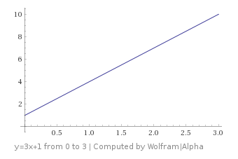
You might remember that the equation of a line is 


In calculus, you learn that the slope m is also the derivative of the function:

The slope / derivative tells you how much is added to y for every 1 you add to x.
Let’s say that you were on this graph at the point 

So, if you want to go downhill to a smaller y value, you know that you need to subtract values from x.
A simpler way to think of this is that you need to subtract the derivative from your x value to make your y value smaller.
That is a core fact that will help guide you through things as they get more difficult: subtract the derivative (later, subtract the gradient) to make your value smaller. The value subtracted is often multiplied by some scalar value to make it move faster or slower.
What happens if you have a more complex function, such as 
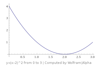
Let’s say that you are on this graph at the point 
The derivative of this function is 
Remembering that we subtract that derivative to go down hill, that means we need to subtract a negative value from our x; aka we need to ADD a value to our x.
As you can see, adding a value to x and making it move to the right does in fact make us go down hill.
The rule works, hooray!
Two Dimensional Gradient Descent
Things do get a little more complex when there’s more than one dimension, but not really that much more complex, so hang in there!
Let’s look at the function


Let’s say that we are at the (x,y) point (1,1) – in the upper right corner – which puts us at 
The answer is PARTIAL derivatives.
First up, we are going to pretend that y is a constant value, and not actually a variable. This will give us the partial derivative for x: 
In this case, the partial derivative of z with respect to x is just: y.
Doing the same thing for the other variable, the partial derivative of z with respect to y is just: x.
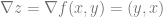
Now that we have partial derivatives for each variable, we put them into a vector. This vector is called the gradient, and has some intimidating notation that looks like this:

For this function, the gradient is:
That makes the gradient at our specific point:
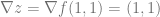
In the last section we saw that the derivative / slope pointed to where the function got larger. The same thing is true of gradients, they point in the direction where the function gets larger too!
So, if we want to go downhill, we need to subtract values from our x and our y to go there. In fact, we know that the steepest way down from our current point is when we subtract the same value from both x and y. This is because the gradient doesn’t just point to where it gets larger, it points to where it gets larger the FASTEST. So, the reverse of the gradient also points to where it gets smaller the fastest.
Pretty cool huh?
You can confirm this visually by looking at the graph of the function.
One last things about slopes, derivatives and gradients before moving on. While they do point in the direction of greatest increase, they are only valid for an infinitely small point on the graph for functions that are non linear. This will be important later when we move in the opposite direction of the gradients, but do so with very small steps to help make sure we find the lowest points on the graph.
Why Gradient Descent?
Why do we want to use gradient descent? Imagine that we have a function:

Sure, we can pick some random starting values for x,y and z, and then use gradient descent to find the smallest w, but who cares?
Let’s give some other names to these variables and see if the value becomes a little more apparent:

Now, by only changing the names of the variables, we can see that we could use gradient descent to find what amount of Armor, Dodge and Resist would make it so our character takes the least amount of damage. This can now tell you how to distribute stat points to a character to get the best results 😛
Note that if you are ever trying to find the highest number possible, instead of the lowest, you can just multiply your function by -1 and do everything else the same way. You could also do gradient ASCENT, but it’s equivalent to multiplying by -1 and doing gradient descent.
Problems
Here are a few common problems you can encounter when doing gradient descent.
- Local minima – when you get to the bottom of a bowl, but it isn’t the deepest bowl.
- Flat derivatives – these make it hard to escape a local area because the derivatives are very small, which will make each movement also very small.
- Discontinuities – The problem space (graph) changes abruptly without warning, making gradient descent do the wrong thing
Here’s an example of a local minima versus a global minima. You can see that depending on where you start on this graph, you might end up in the deeper bowl, or the shallower bowl if your only rule is “move downhill”.

(Image from wikipedia By KSmrq – http://commons.wikimedia.org/wiki/File:Extrema_example.svg, GFDL 1.2, https://commons.wikimedia.org/w/index.php?curid=6870865)
Here’s an example of a flat derivative. You can imagine that if you were at x=1, that you could see that the derivative would tell you to go to the left to decrease the y value, but it’s a very, very small number. This is a problem because it’s common to multiply the derivative or gradient by a multiplier before subtracting it, so you’d only take a very small step towards the goal.
It’s also possible to hit a perfectly flat derivative, which will be exactly 0. In this case, no matter how big or small of a number you multiply the derivative by, you won’t move AT ALL!
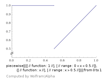
Below is a discontinuous function where if x is less than 0.5, the value is 1, otherwise the value is x. This essentially shows you what happens when you use if statements in differentiable programming. If you start on the right side, it’s going to correctly tell you that you should move left to improve your score. However, it’ll keep telling you to move left, until you get to x being less than 0.5, at which point your score will suddenly get a lot worse and your derivative will become 0. You will now be stuck!
There are ways to deal with these problems, but they are deep topics. If nothing else, you should know these problems exist, so you can know when they are affecting you, and/or why you should avoid them if you have a choice.
What If I Want to Avoid Calculus?
Let’s say that you don’t get a kick out of calculating all these partial derivatives. Or, more pragmatically, you don’t want to sit down and manually calculate the gradient function of some generic C++ code!
I have some great news for you.
While we do need partial derivatives for our gradients, we aren’t going to have to do all this calculus to get them!
Here are a few other ways to get partial derivatives:
- Finite Differences – Conceptually super simple, but slow to calculate and not always very precise. More info: Finite Differences
- Backpropagation – What neural networks use. Also called backwards mode automatic differentiation. Fast but a bit complex mentally. I linked this already but for more info: How to Train Neural Networks With Backpropagation
- Dual Numbers – Also called forward mode automatic differentiation. Not as fast as backwards mode, but in the same neighborhood for speed. Super, super convinient and awesome for programmers. I love these. More info: Dual Numbers & Automatic Differentiation
Care to guess which one we are going to use? Yep, Dual Numbers!
In a nutshell, if you have code that uses floats, you can change it to use a templated type instead. Then, you put dual numbers through your code instead of floats. The output you get will be the specific value output from your code, but also the GRADIENT of your code at that value. Even better, this isn’t a numerical method (it’s not an approximation), it’s analytical (it’s exact).
That is seriously all there is to it. Dual numbers are amazing!
Since you made the code templated, you can still use it for floats when you don’t want or need the gradient.
Differentiable Programming / Gradient Descent Skeleton
Here’s the general skeleton we are going to be following for using gradient descent with our differentiable program.
- Initialize the parameters to random (but valid) values, storing them in dual numbers.
- Run the code that does our work, taking dual numbers as input for the parameters of how it does the work.
- Put the result (which is dual numbers) into a scoring function to give us a score. Usually the score is such that smaller numbers are better. If not, just multiply the score by -1 so it is.
- Since we did the work and calculated the score using dual numbers, we now have a gradient which describes how we need to adjust the parameters to make our score better.
- Adjust our parameters using the gradient and go back to step 2. Repeating until whatever exit condition we want is hit: maybe when a certain number of iterations happen, or maybe when our score gets below a certain value.
That’s our game plan. Let’s dive into the specific problem we are going to be attacking.
Searching For an Ideal Dithering Pattern
Here is the problem we want to tackle:
We want to find a 3×3 dithering pattern such that when we use it to dither an image (by repeating the 3×3 pattern over and over across the image), and then blur the result by a specific amount, that it’s as close as possible to the original image being blurred by that same amount.
That sounds a bit challenging right? It’s not actually that bad, don’t worry (:
The steps the code has to do (differentiably) are:
- Dither the source image
- Blur the results
- Blur the source image
- Calculate a score for how similar they are
- Use all this with Gradient Descent to optimize the dither pattern
Once again, we need to do this stuff differentiably, using dual numbers, so that we get a gradient for how to modify the dither pattern to better our score.
Step 1 – Dither Source Image
Dithering an image is a pretty simple process.
We are going to be dithering it such that we take a greyscale image as input and convert it to a black and white image using the dither pattern.
(If you are starting with a color image, this shows how to convert it to greyscale: Converting RGB to Grayscale)
For every pixel (x,y) in the source image, you look at pixel (x%3, y%3) in the dither pattern, and if the dither pattern pixel is less than the source, you write a black pixel out, else you write a white pixel out.
if (sourcePixel(x,y) < ditherPixel(x%3, y%3))
    pixelOut(x,y) = 0.0;
else
    pixelOut(x,y) = 1.0;
There’s a problem though… this is a branch, which makes a discontinuity, which will make it so we can’t have good derivatives to help us get to the goal.
Another way to write the dithering operation above is to write it like this:
difference = ditherPixel(x%3, y%3) - sourcePixel(x,y);
pixelOut(x,y) = step(difference);
Where “step” is the “heaviside step function”, which is 1 if x >= 0, otherwise is 0.

(Image from Wikipedia By Omegatron (Own work) [CC BY-SA 3.0 (https://creativecommons.org/licenses/by-sa/3.0) or GFDL (http://www.gnu.org/copyleft/fdl.html)%5D, via Wikimedia Commons)
That got rid of the branch (if statement), but we still have a discontinuous function.
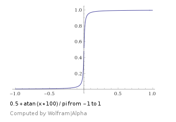
Luckily we can approximate a step function with other functions. I decided to use the formula 
Unfortunately, I found that my results weren’t that good, so i switched it to 
This function does have the problem of having flat derivatives, but I found that it worked pretty well anyways. The flat derivatives don’t seem to be a big problem in this case luckily.
To put it all together, the differentiable version of dithering a pixel that I use looks like this:
difference = ditherPixel(x%3, y%3) - sourcePixel(x,y);
pixelOut(x,y) = 0.5+atan(10000.0f * difference) / pi;
As input to this dithering process, we take:
- The source image
- a 3×3 dither pattern, where each pixel is a dual number
As output this dithering process gives us:
- A dithered image that is converted to black and white (either a 1.0 or 0.0 value per pixel)
- It’s the same size as the source image
- Each pixel is a dual number with 9 derivatives. There is one derivative per dither pixel.
Step 2 – Blur the Results
Blurring the results of the dither wasn’t that difficult. I used a Gaussian blur, but other blurs could be used easily.
I had some Gaussian blur code laying around (from this blog post: Gaussian Blur) and I converted it to using a templated type instead of floats/pixels where appropriate, also making sure there were no branches or anything discontinuous.
It turned out there wasn’t a whole lot to fix up here luckily so wasn’t too difficult.
This allowed me to take the dithered results which are a dual number per pixel, and do a Gaussian blur on them, preserving and correctly modifying the gradient (derivatives) as it did the Blur.
Step 3 – Blur the Source Image
Blurring the source image was easy since the last step made a generic gaussian blur function. I used the generic Gaussian blur function to blur the image. This doesn’t need to be done as dual numbers, so it was regular pixels in and regular pixels out.
You might wonder why this part doesn’t need to be done as dual numbers.
The simple answer is because these values are in no way dependant on the dither pattern (which are what we are tracking with the derivatives).
The more mathematical explanation is that you could in fact consider these dual numbers, which just have a gradient of zero because they are essentially constants that have nothing to do (yet) with the parameters of the function. The gradient would just implicitly be zero, like any other constant value you might introduce to the function.
Step 4 – Calculating a Similarity Score
Next up I needed to calculate a similarity score between the dithered then blurred results (which is made up of dual numbers), and the source image which was blurred (and is made up of regular pixels).
The similarity score I went with is just MSE or “Mean Squared Error”.
To calculate MSE, for every pixel you do this:
error = ditheredBlurredImage(x,y) - blurredImage(x,y);
errorSquared = error * error;
After you have the squared error for every pixel, you just take the average of them to get the MSE.
An interesting thing about MSE is that because errors are squared, it will favor smaller errors much more than larger errors, which is a nice property.
A not so nice property about MSE is that it might decide something is a small difference mathematically even though a human would decide that it was a huge difference perceptually. The reverse is also true. Despite this, I chose it because it is simple and I ended up getting decent results with it.
If you want to go down the rabbit hole of looking at “perceptual similarity scores of images” check out these links:
- SSIM – http://www.cns.nyu.edu/~lcv/ssim/
- GMSD – https://arxiv.org/ftp/arxiv/papers/1308/1308.3052.pdf
- Multiple Scale SSIM -http://www.cns.nyu.edu/~zwang/files/papers/msssim.pdf
After this step, we have an MSE value which says how similar the images are. A lower value means lower average squared error, so lower numbers are indeed better.
What else is nice is that the MSE value is a dual number with a gradient that has the 9 partial derivatives that describe how much the MSE changes as you adjust each parameter.
That gradient tells us how to adjust the parameters (the 3×3 dither pixels!) to lower the MSE!
Step 5 – Putting it All Together
Now it’s time to put all of this together and use gradient descent to make our dither pattern better.
Here’s how the program operates:
- Initialize the 3×3 dither pattern to random values, setting the derivatives to 1.0 in the gradient, for the variable that they represent.
- do 1000 iterations of this loop:
- Dither and blur the source image
- Calculate MSE of this result compared to the source image blurred
- Using the gradient from the MSE value, subtract the respective partial derivative from each of the pixels in the dither pattern, but scaling the partial derivative by a “learning rate”.
- Output the best result found
The learning rate starts at 3.0 at loop iteration 0, but decays with each iteration, down to 0.1 at iteration 999. It starts above 1 to help escape local minima, and uses a very small rate at the end to try and get deeper into whatever minimum it has found.
After adjusting the dither pattern pixels, I clamp them to be between 0 and 1.
Something else I ought to mention is that while I’m doing the gradient descent, I keep track of the best scoring dither pattern seen.
This way, after the 1000 iterations are up, if we ever saw anything better than where we are at currently, we just use that instead of the final result.
Presumably, if you tune your parameters (learning rate, iterations, etc!) correctly, this won’t come up often, but it’s always a possibility that your final state is not the best state encountered, so this is a nice way to get better results more often.
Results
Did you notice that I called this post “searching for an ideal dither pattern” instead of “finding an ideal dither pattern”? (:
The results are decent, but I know they could be better. Even so, I think the techniques talked about here are a good start going down the path of differentiable programming, and similar topics.
Here are some results I was able to get with the code. Click to see the full size images. The shrunken down images have aliasing issues.
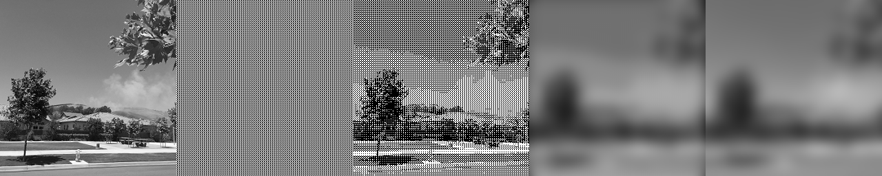
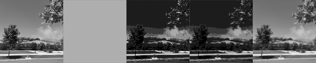
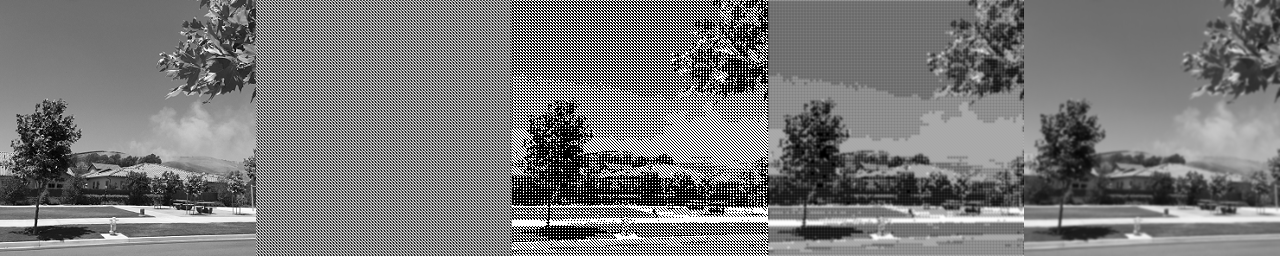
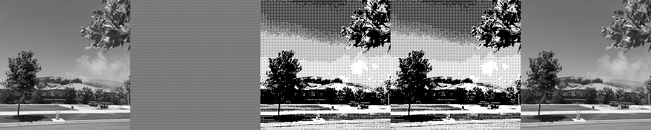
The images left to right are: The original, the dither pattern used (repeated), the dithered image, the blurred dither image, and lastly the blurred original image. The program aims to make the last two images look as close as possible as it can, using MSE as the metric for how close they are.
Here is the starting state of using a Gaussian blur with a sigma of 10:
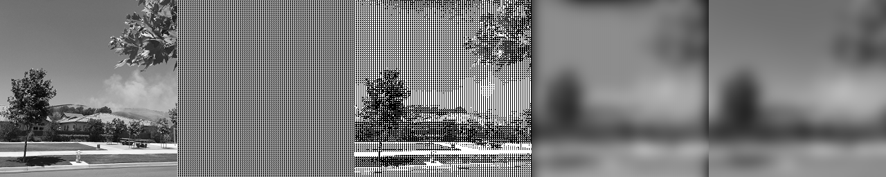
Here it is after the 1000 iterations of gradient descent. Notice the black blob at the top is gone compared to where it started.
Here’s the starting state when using a Gaussian blur sigma of 1:
And here it is after 1000 iterations, which is pretty decent results:
Lastly, here it is with no blurring whatsoever:
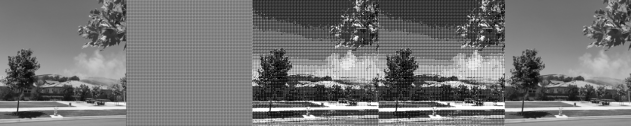
And after 1000 iterations, I think it actually looks worse!
Using no blur at all makes for some really awful results. The blur gives the algorithm more freedom on how it can succeed, whereas with no blur, there is a lot less wiggle room for finding a solution.
Another benefit of using the blur before MSE calculation is that a blur is a low pass filter. That means that higher frequencies are gone before the MSE calculation. The result of this is that the algorithm will favor results which are closer to blue noise dithering. Pretty neat right?!
Closing
I hope you enjoyed this journey through differentiable programming and gradient descent, and I hope you were able to follow along.
Here are some potentially interesting things to do beyond what we talked about here:
- Have it learn from a set of images, instead of only this single image. This should help prevent “over fitting” and let it find a dither pattern which works well for all images instead of just this one specific image.
- Use a separate set of images to gauge the accuracy of the result that weren’t used as part of the training, to help prove that it really hasn’t overfit the training data.
- Try applying “small corruption” in the learning to help prevent overfitting or getting stuck in local minima – one idea would be to have some percentage chance per derivative that you don’t apply the change to the dither pattern pixel. This would add some randomness to the gradient descent instead of it only being down the steepest direction all of the time.
- Instead of optimizing the dithering patterns, you could make a formula that generated the dithering patterns, and instead optimize the coefficients / terms of that formula. If you get good results, you’ll end up with a formula you can use for dithering instead of a pattern, which might be nice for the case of avoiding a texture read in a pixel shader to do the dithering.
I’m not a data scientist or machine learning expert by any means, so there are plenty of improvements to be made. There is a lot of overlap with what is being done here and other algorithms – both in the machine learning realm and outside of the machine learning realm.
For one, you can use Newton’s method for gradient descent. It can find minima faster by using the second derivative in the calculations as well.
However, this algorithm is almost purely “exploitative” in that wherever you start with your parameters, it will try to go from there to the deepest point in whatever valley it’s already in. Some other types of algorithms differ from this in that they are more “explorative” and try to find other valleys, but aren’t always as good at finding the deepest part of the valleys that they do find. More explorative algorithms include simulated annealing, differential evolution, and genetic algorithms.
If you enjoyed this post, check out this book for deeper details on algorithms relating to gradient descent (simulated annealing, genetic algorithms, etc!). It’s a very good book and very easy to read!
Essentials of Metaheuristics
Any corrections to what i’ve said, the code, or suggestions for improvements, please let me know by leaving a comment here, or hitting me up on twitter: https://twitter.com/Atrix256
