This post is an attempt to demystify backpropagation, which is the most common method for training neural networks. This post is broken into a few main sections:
- Explanation
- Working through examples
- Simple sample C++ source code using only standard includes
- Links to deeper resources to continue learning
Let’s talk about the basics of neural nets to start out, specifically multi layer perceptrons. This is a common type of neural network, and is the type we will be talking about today. There are other types of neural networks though such as convolutional neural networks, recurrent neural networks, Hopfield networks and more. The good news is that backpropagation applies to most other types of neural networks too, so what you learn here will be applicable to other types of networks.
Basics of Neural Networks
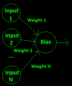
A neural network is made up layers.
Each layer has some number of neurons in it.
Every neuron is connected to every neuron in the previous and next layer.
Below is a diagram of a neural network, courtesy of wikipedia. Every circle is a neuron. This network takes 3 floating point values as input, passes them through 4 neurons in a hidden layer and outputs two floating point values. The hidden layer neurons and the output layer neurons do processing of the values they are giving, but the input neurons do not.

To calculate the output value of a single neuron, you multiply every input into that neuron by a weight for that input, sum them up, and add a bias that is set for the neuron. This “weighted input” value is fed into an activation function and the result is the output value of that neuron. Here is a diagram for a single neuron:
The code for calculating the output of a single neuron could look like this:
float weightedInput = bias;

for (int i = 0; i < inputs.size(); ++i)
  weightedInput += inputs[i] * weights[i];

float output = Activation(weightedInput);
To evaluate an entire network of neurons, you just repeat this process for all neurons in the network, going from left to right (from input to output).
Neural networks are basically black boxes. We train them to give specific ouputs when we give them specific inputs, but it is often difficult to understand what it is that they’ve learned, or what part of the data they are picking up on.
Training a neural network just means that we adjust the weight and bias values such that when we give specific inputs, we get the desired outputs from the network. Being able to figure out what weights and biases to use can be tricky, especially for networks with lots of layers and lots of neurons per layer. This post talks about how to do just that.
Regarding training, there is a funny story where some people trained a neural network to say whether or not a military tank was in a photograph. It had a very high accuracy rate with the test data they trained it with, but when they used it with new data, it had terrible accuracy. It turns out that the training data was a bit flawed. Pictures of tanks were all taken on a sunny day, and the pictures without tanks were taken on a cloudy day. The network learned how to detect whether a picture was of a sunny day or a cloudy day, not whether there was a tank in the photo or not!
This is one type of pitfall to watch out for when dealing with neural networks – having good training data – but there are many other pitfalls to watch out for too. Architecting and training neural networks is quite literally an art form. If it were painting, this post would be teaching you how to hold a brush and what the primary colors are. There are many, many techniques to learn beyond what is written here to use as tools in your toolbox. The information in this post will allow you to succeed in training neural networks, but there is a lot more to learn to get higher levels of accuracy from your nets!
Neural Networks Learn Using Gradient Descent
Let’s take a look at a simple neural network where we’ve chosen random values for the weights and the bias:
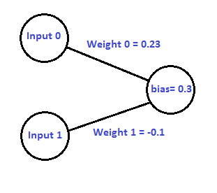
If given two floating point inputs, we’d calculate the output of the network like this:

Plugging in the specific values for the weights and biases, it looks like this:

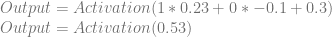
Let’s say that we want this network to output a zero when we give an input of 1,0, and that we don’t care what it outputs otherwise. We’ll plug 1 and 0 in for Input0 and Input1 respectively and see what the output of the network is right now:
For the activation function, we are going to use a common one called the sigmoid activation function, which is also sometimes called the logistic activation function. It looks like this:

Without going into too much detail, the reason why sigmoid is so commonly used is because it’s a smoother and differentiable version of the step function.
Applying that activation function to our output neuron, we get this:
So, we plugged in 1 and 0, but instead of getting a 0 out, we got 0.6295. Our weights and biases are wrong, but how do we correct them?
The secret to correcting our weights and biases is whichever of these terms seem least scary to you: slopes, derivatives, gradients.
If “slope” was the least scary term to you, you probably remember the line formula  and that the m value was the “rise over run” or the slope of the line. Well believe it or not, that’s all a derivative is. A derivative is just the slope of a function at a specific point on that function. Even if a function is curved, you can pick a point on the graph and get a slope at that point. The notation for a derivative is
  , which literally means “change in y divided by change in x”, or “delta y divided by delta x”, which is literally rise over run.
In the case of a linear function (a line), it has the same derivative over the entire thing, so you can take a step size of any size on the x axis and multiply that step size by to figure out how much to add or subtract from y to stay on the line.
In the case of a non linear function, the derivative can change from one point to the next, so this slope is only guaranteed to be accurate for an infinitely small step size. In practice, people just often use “small” step sizes and calling it good enough, which is what we’ll be doing momentarily.
Now that you realize you already knew what a derivative is, we have to talk about partial derivatives. There really isn’t anything very scary about them and they still mean the exact same thing – they are the slope! They are even calculated the exact same way, but they use a fancier looking d in their notation:  .
.
The reason partial derivatives even exist is because if you have a function of multiple variables like  , you have two variables that you can take the derivative of. You can calculate
  and
and  . The first value tells you how much the z value changes for a change in x, the second value tells you how much the z value changes for a change in y.
By the way, if you are curious, the partial derivatives for that function above are below. When calculating partial derivatives, any variable that isn’t the one you care about, you just treat as a constant and do normal derivation.

If you put both of those values together into a vector  you have what is called the gradient vector.
The gradient vector has an interesting property, which is that it points in the direction that makes the function output grow the most. Basically, if you think of your function as a surface, it points up the steepest direction of the surface, from the point you evaluated the function at.
We are going to use that property to train our neural network by doing the following:
- Calculate the gradient of a function that describes the error in our network. This means we will have the partial derivatives of all the weights and biases in the network.
- Multiply the gradient by a small “learning rate” value, such as 0.05
- Subtract these scaled derivatives from the weights and biases to decrease the error a small amount.
This technique is called steepest gradient descent (SGD) and when we do the above, our error will decrease by a small amount. The only exception is that if we use too large of a learning rate, it’s possible that we make the error grow, but usually the error will decrease.
We will do the above over and over, until either the error is small enough, or we’ve decided we’ve tried enough iterations that we think the neural network is never going to learn the things we want to teach it. If the network doesn’t learn, it means it needs to be re-architected with a different structure, different numbers of neurons and layers, different activation functions, etc. This is part of the “art” that I mentioned earlier.
Before moving on, there is one last thing to talk about: global minimums vs local minimums.
Imagine that the function describing the error in our network is visualized as bumpy ground. When we initialize our weights and biases to random numbers we are basically just choosing a random location on the ground to start at. From there, we act like a ball, and just roll down hill from wherever we are. We are definitely going to get to the bottom of SOME bump / hole in the ground, but there is absolutely no reason to except that we’ll get to the bottom of the DEEPEST bump / hole.
The problem is that SGD will find a LOCAL minimum – whatever we are closest too – but it might not find the GLOBAL minimum.
In practice, this doesn’t seem to be too large of a problem, at least for people casually using neural nets like you and me, but it is one of the active areas of research in neural networks: how do we do better at finding more global minimums?
You might notice the strange language I’m using where I say we have a function that describes the error, instead of just saying we use the error itself. The function I’m talking about is called the “cost function” and the reason for this is that different ways of describing the error give us different desirable properties.
For instance, a common cost function is to use mean squared error of the actual output compared to the desired output.
For a single training example, you plug the input into the network and calculate the output. You then plug the actual output and the target output into the function below:

In other words, you take the vector of the neuron outputs, subtract it from the actual output that we wanted, calculate the length of the resulting vector and square it. This gives you the squared error.
The reason we use squared error in the cost function is because this way error in either direction is a positive number, so when gradient descent does it’s work, we’ll find the smallest magnitude of error, regardless of whether it’s positive or negative amounts. We could use absolute value, but absolute value isn’t differentiable, while squaring is.
To handle calculating the cost of multiple inputs and outputs, you just take the average of the squared error for each piece of training data. This gives you the mean squared error as the cost function across all inputs. You also average the derivatives to get the combined gradient.
More on Training
Before we go into backpropagation, I want to re-iterate this point: Neural Networks Learn Using Gradient Descent.
All you need is the gradient vector of the cost function, aka the partial derivatives of all the weights and the biases for the cost.
Backpropagation gets you the gradient vector, but it isn’t the only way to do so!
Another way to do it is to use dual numbers which you can read about on my post about them: Multivariable Dual Numbers & Automatic Differentiation.
Using dual numbers, you would evaluate the output of the network, using dual numbers instead of floating point numbers, and at the end you’d have your gradient vector. It’s not quite as efficient as backpropagation (or so I’ve heard, I haven’t tried it), but if you know how dual numbers work, it’s super easy to implement.
Another way to get the gradient vector is by doing so numerically using finite differences. You can read about numerical derivatives on my post here: Finite Differences
Basically what you would do is if you were trying to calculate the partial derivative of a weight, like  , you would first calculate the cost of the network as usual, then you would add a small value to Weight0 and evaluate the cost again. You subtract the new cost from the old cost, and divide by the small value you added to Weight0. This will give you the partial derivative for that weight value. You’d repeat this for all your weights and biases.
Since realistic neural networks often have MANY MANY weights and biases, calculating the gradient numerically is a REALLY REALLY slow process because of how many times you have to run the network to get cost values with adjusted weights. The only upside is that this method is even easier to implement than dual numbers. You can literally stop reading and go do this right now if you want to 😛
Lastly, there is a way to train neural networks which doesn’t use derivatives or the gradient vector, but instead uses the more brute force-ish method of genetic algorithms.
Using genetic algorithms to train neural networks is a huge topic even to summarize, but basically you create a bunch of random networks, see how they do, and try combining features of networks that did well. You also let some of the “losers” reproduce as well, and add in some random mutation to help stay out of local minimums. Repeat this for many many generations, and you can end up with a well trained network!
Here’s a fun video visualizing neural networks being trained by genetic algorithms: Youtube: Learning using a genetic algorithm on a neural network
Backpropagation is Just the Chain Rule!
Going back to our talk of dual numbers for a second, dual numbers are useful for what is called “forward mode automatic differentiation”.
Backpropagation actually uses “reverse mode automatic differentiation”, so the two techniques are pretty closely tied, but they are both made possible by what is known as the chain rule.
The chain rule basically says that if you can write a derivative like this:

That you can also write it like this:
That might look weird or confusing, but since we know that derivatives are actual values, aka actual ratios, aka actual FRACTIONS, let’s think back to fractions for a moment.

So far so good? Now let’s choose some number out of the air – say, 5 – and do the same thing we did with the chain rule

Due to doing the reverse of cross cancellation, we are able to inject multiplicative terms into fractions (and derivatives!) and come up with the same answer.
Ok, but who cares?
Well, when we are evaluating the output of a neural network for given input, we have lots of equations nested in each other. We have neurons feeding into neurons feeding into neurons etc, with the logistic activation function at each step.
Instead of trying to figure out how to calculate the derivatives of the weights and biases for the entire monster equation (it’s common to have hundreds or thousands of neurons or more!), we can instead calculate derivatives for each step we do when evaluating the network and then compose them together.
Basically, we can break the problem into small bites instead of having to deal with the equation in it’s entirety.
Instead of calculating the derivative of how a specific weight affects the cost directly, we can instead calculate these:
- dCost/dOutput: The derivative of how a neuron’s output affects cost
- dOutput/dWeightedInput: The derivative of how the weighted input of a neuron affects a neuron’s output
- dWeightedInput/dWeight: The derivative of how a weight affects the weighted input of a neuron
Then, when we multiply them all together, we get the real value that we want:
dCost/dOutput * dOutput/dWeightedInput * dWeightedInput/dWeight = dCost/dWeight
Now that we understand all the basic parts of back propagation, I think it’d be best to work through some examples of increasing complexity to see how it all actually fits together!
Backpropagation Example 1: Single Neuron, One Training Example
This example takes one input and uses a single neuron to make one output. The neuron is only trained to output a 0 when given a 1 as input, all other behavior is undefined. This is implemented as the Example1() function in the sample code.

Backpropagation Example 2: Single Neuron, Two Training Examples
Let’s start with the same neural network from last time:
This time, we are going to teach it not only that it should output 0 when given a 1, but also that it should output 1 when given a 0.
We have two training examples, and we are training the neuron to act like a NOT gate. This is implemented as the Example2() function in the sample code.
The first thing we do is calculate the derivatives (gradient vector) for each of the inputs.
We already calculated the “input 1, output 0” derivatives in the last example:
If we follow the same steps with the “input 0, output 1” training example we get these:
To get the actual derivatives to train the network with, we just average them!
From there, we do the same adjustments as before to the weight and bias values to get a weight of 0.2631 and a bias of 0.4853.
If you are wondering how to calculate the cost, again you just take the cost of each training example and average them. Adjusting the weight and bias values causes the cost to drop from 0.1547 to 0.1515, so we have made progress.
It takes 10 times as many iterations with these two training examples to get the same level of error as it did with only one training example though.
As we saw in the last example, after 10,000 iterations, the error was 0.007176.
In this example, after 100,000 iterations, the error is 0.007141. At that point, weight is -9.879733 and bias is 4.837278
Backpropagation Example 3: Two Neurons in One Layer
Here is the next example, implemented as Example3() in the sample code. Two input neurons feed to two neurons in a single layer giving two outputs.
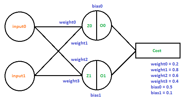
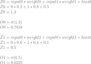
Let’s look at how we’d calculate the derivatives needed to train this network using the training example that when we give the network 01 as input that it should give out 10 as output.
First comes the forward pass where we calculate the network’s output when we give it 01 as input.
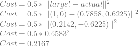
Next we calculate a cost. We don’t strictly need to do this step since we don’t use this value during backpropagation, but this will be useful to verify that we’ve improved things after an iteration of training.
Now we begin the backwards pass to calculate the derivatives that we’ll need for training.
Let’s calculate dCost/dZ0 aka the error in neuron 0. We’ll do this by calculating dCost/dO0, then dO0/dZ0 and then multiplying them together to get dCost/dZ0. Just like before, this is also the derivative for the bias of the neuron, so this value is also dCost/dBias0.
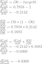
We can use dCost/dZ0 to calculate dCost/dWeight0 and dCost/dWeight1 by multiplying it by dZ0/dWeight0 and dZ0/dWeight1, which are input0 and input1 respectively.

Next we need to calculate dCost/dZ1 aka the error in neuron 1. We’ll do this like before. We’ll calculate dCost/dO1, then dO1/dZ1 and then multiplying them together to get dCost/dZ1. Again, this is also the derivative for the bias of the neuron, so this value is also dCost/dBias1.
Just like with neuron 0, we can use dCost/dZ1 to calculate dCost/dWeight2 and dCost/dWeight3 by multiplying it by dZ1/dWeight2 and dZ1/dWeight2, which are input0 and input1 respectively.
After using these derivatives to update the weights and biases with a learning rate of 0.5, they become:
Weight0 = 0.2
Weight1 = 0.818
Weight2 = 0.6
Weight3 = 0.3269
Bias0 = 0.518
Bias1 = 0.0269
Using these values, the cost becomes 0.1943, which dropped from 0.2167, so we have indeed made progress with our learning!
Interestingly, it takes about twice as many trainings as example 1 to get a similar level of error. In this case, 20,000 iterations of learning results in an error of 0.007142.
If we have the network learn the four patterns below instead:
00 = 00
01 = 10
10 = 10
11 = 11
It takes 520,000 learning iterations to get to an error of 0.007223.
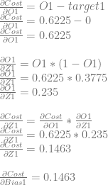
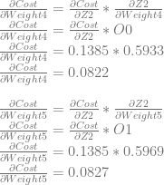
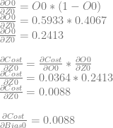
Backpropagation Example 4: Two Layers, Two Neurons Each
This is the last example, implemented as Example4() in the sample code. Two input neurons feed to two neurons in a hidden layer, feeding into two neurons in the output layer giving two outputs. This is the exact same network that is walked through on this page which is also linked to at the end of this post: A Step by Step Backpropagation Example

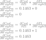
First comes the forward pass where we calculate the network’s output. We’ll give it 0.05 and 0.1 as input, and we’ll say our desired output is 0.01 and 0.99.

Next we calculate the cost, taking O2 and O3 as our actual output, and 0.01 and 0.99 as our target (desired) output.
Now we start the backward pass to calculate the derivatives for training.
Neuron 2
First we’ll calculate dCost/dZ2 aka the error in neuron 2, remembering that the value is also dCost/dBias2.
We can use dCost/dZ2 to calculate dCost/dWeight4 and dCost/dWeight5.
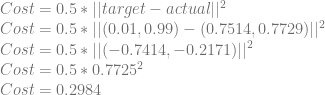
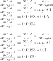
Neuron 3
Next we’ll calculate dCost/dZ3 aka the error in neuron 3, which is also dCost/dBias3.
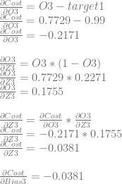
We can use dCost/dZ3 to calculate dCost/dWeight6 and dCost/dWeight7.
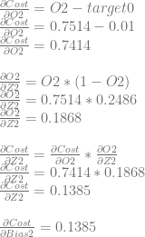
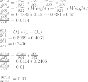
Neuron 0
Next, we want to calculate dCost/dO0, but doing that requires us to do something new. Neuron 0 affects both neuron 2 and neuron 3, which means that it affects the cost through those two neurons as well. That means our calculation for dCost/dO0 is going to be slightly different, where we add the derivatives of both paths together. Let’s work through it:
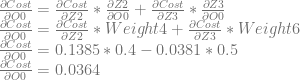
We can then continue and calculate dCost/dZ0, which is also dCost/dBias0, and the error in neuron 0.
We can use dCost/dZ0 to calculate dCost/dWeight0 and dCost/dWeight1.
Neuron 1
We are almost done, so hang in there. For our home stretch, we need to calculate dCost/dO1 similarly as we did for dCost/dO0, and then use that to calculate the derivatives of bias1 and weight2 and weight3.
Lastly, we will use dCost/dZ1 to calculate dCost/dWeight2 and dCost/dWeight3.
Backpropagation Done
Phew, we have all the derivatives we need now.
Here’s our new weights and biases using a learning rate of 0.5:
Weight0 = 0.15 – (0.5 * 0.0004) = 0.1498
Weight1 = 0.2 – (0.5 * 0.0009) = 0.1996
Weight2 = 0.25 – (0.5 * 0.0005) = 0.2498
Weight3 = 0.3 – (0.5 * 0.001) = 0.2995
Weight4 = 0.4 – (0.5 * 0.0822) = 0.3589
Weight5 = 0.45 – (0.5 * 0.0827) = 0.4087
Weight6 = 0.5 – (0.5 * -0.0226) = 0.5113
Weight7 = 0.55 – (0.5 * -0.0227) = 0.5614
Bias0 = 0.35 – (0.5 * 0.0088) = 0.3456
Bias1 = 0.35 – (0.5 * 0.01) = 0.345
Bias2 = 0.6 – (0.5 * 0.1385) = 0.5308
Bias3 = 0.6 – (0.5 * -0.0381) = 0.6191
Using these new values, the cost function value drops from 0.2984 to 0.2839, so we have made progress!
Interestingly, it only takes 5,000 iterations of learning for this network to reach an error of 0.007157, when it took 10,000 iterations of learning for example 1 to get to 0.007176.
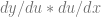
Before moving on, take a look at the weight adjustments above. You might notice that the derivatives for the weights are much smaller for weights 0,1,2,3 compared to weights 4,5,6,7. The reason for this is because weights 0,1,2,3 appear earlier in the network. The problem is that earlier layer neurons don’t learn as fast as later layer neurons and this is caused by the nature of the neuron activation functions – specifically, that the sigmoid function has a long tail near 0 and 1 – and is called the “vanishing gradient problem”. The opposite effect can also happen however, where earlier layer gradients explode to super huge numbers, so the more general term is called the “unstable gradient problem”. This is an active area of research on how to address, and this becomes more and more of a problem the more layers you have in your network.
You can use other activation functions such as tanh, identity, relu and others to try and get around this problem. If trying different activation functions, the forward pass (evaluation of a neural network) as well as the backpropagation of error pass remain the same, but of course the calculation for getting O from Z changes, and of course, calculating the derivative deltaO/deltaZ becomes different. Everything else remains the same.
Check the links at the bottom of the post for more information about this!
Sample Code
Below is the sample code which implements all the back propagation examples we worked through above.
Note that this code is meant to be readable and understandable. The code is not meant to be re-usable or highly efficient.
A more efficient implementation would use SIMD instructions, multithreading, stochastic gradient descent, and other things.
It’s also useful to note that calculating a neuron’s Z value is actually a dot product and an addition and that the addition can be handled within the dot product by adding a “fake input” to each neuron that is a constant of 1. This lets you do a dot product to calculate the Z value of a neuron, which you can take further and combine into matrix operations to calculate multiple neuron values at once. You’ll often see neural networks described in matrix notation because of this, but I have avoided that in this post to try and make things more clear to programmers who may not be as comfortable thinking in strictly matrix notation.
#include <stdio.h>
#include <array>

// Nonzero value enables csv logging.
#define LOG_TO_CSV_NUMSAMPLES() 50

// ===== Example 1 - One Neuron, One training Example =====

void Example1RunNetwork (
	float input, float desiredOutput,
	float weight, float bias,
	float& error, float& cost, float& actualOutput,
	float& deltaCost_deltaWeight, float& deltaCost_deltaBias, float& deltaCost_deltaInput
) {
	// calculate Z (weighted input) and O (activation function of weighted input) for the neuron
	float Z = input * weight + bias;
	float O = 1.0f / (1.0f + std::exp(-Z));

	// the actual output of the network is the activation of the neuron
	actualOutput = O;

	// calculate error
	error = std::abs(desiredOutput - actualOutput);

	// calculate cost
	cost = 0.5f * error * error;

	// calculate how much a change in neuron activation affects the cost function
	// deltaCost/deltaO = O - target
	float deltaCost_deltaO = O - desiredOutput;

	// calculate how much a change in neuron weighted input affects neuron activation
	// deltaO/deltaZ = O * (1 - O)
	float deltaO_deltaZ = O * (1 - O);


	// calculate how much a change in a neuron's weighted input affects the cost function.
	// This is deltaCost/deltaZ, which equals deltaCost/deltaO * deltaO/deltaZ
	// This is also deltaCost/deltaBias and is also refered to as the error of the neuron
	float neuronError = deltaCost_deltaO * deltaO_deltaZ;
	deltaCost_deltaBias = neuronError;

	// calculate how much a change in the weight affects the cost function.
	// deltaCost/deltaWeight = deltaCost/deltaO * deltaO/deltaZ * deltaZ/deltaWeight
	// deltaCost/deltaWeight = neuronError * deltaZ/deltaWeight
	// deltaCost/deltaWeight = neuronError * input
	deltaCost_deltaWeight = neuronError * input;


	// As a bonus, calculate how much a change in the input affects the cost function.
	// Follows same logic as deltaCost/deltaWeight, but deltaZ/deltaInput is the weight.
	// deltaCost/deltaInput = neuronError * weight
	deltaCost_deltaInput = neuronError * weight;
}

void Example1 ()
{
	#if LOG_TO_CSV_NUMSAMPLES() > 0
		// open the csv file for this example
		FILE *file = fopen("Example1.csv","w+t");
		if (file != nullptr)
			fprintf(file, ""training index","error","cost","weight","bias","dCost/dWeight","dCost/dBias","dCost/dInput"n");
	#endif

	// learning parameters for the network
	const float c_learningRate = 0.5f;
	const size_t c_numTrainings = 10000;

	// training data
	// input: 1, output: 0
	const std::array<float, 2> c_trainingData = {1.0f, 0.0f};

	// starting weight and bias values
	float weight = 0.3f;
	float bias = 0.5f;

	// iteratively train the network
	float error = 0.0f;
	for (size_t trainingIndex = 0; trainingIndex < c_numTrainings; ++trainingIndex)
	{
		// run the network to get error and derivatives
		float output = 0.0f;
		float cost = 0.0f;
		float deltaCost_deltaWeight = 0.0f;
		float deltaCost_deltaBias = 0.0f;
		float deltaCost_deltaInput = 0.0f;
		Example1RunNetwork(c_trainingData[0], c_trainingData[1], weight, bias, error, cost, output, deltaCost_deltaWeight, deltaCost_deltaBias, deltaCost_deltaInput);

		#if LOG_TO_CSV_NUMSAMPLES() > 0
			const size_t trainingInterval = (c_numTrainings / (LOG_TO_CSV_NUMSAMPLES() - 1));
			if (file != nullptr && (trainingIndex % trainingInterval == 0 || trainingIndex == c_numTrainings - 1))
			{
				// log to the csv
				fprintf(file, ""%zi","%f","%f","%f","%f","%f","%f","%f",n", trainingIndex, error, cost, weight, bias, deltaCost_deltaWeight, deltaCost_deltaBias, deltaCost_deltaInput);
			}
		#endif

		// adjust weights and biases
		weight -= deltaCost_deltaWeight * c_learningRate;
		bias -= deltaCost_deltaBias * c_learningRate;
	}

	printf("Example1 Final Error: %fn", error);

	#if LOG_TO_CSV_NUMSAMPLES() > 0
		if (file != nullptr)
			fclose(file);
	#endif
}

// ===== Example 2 - One Neuron, Two training Examples =====

void Example2 ()
{
	#if LOG_TO_CSV_NUMSAMPLES() > 0
		// open the csv file for this example
		FILE *file = fopen("Example2.csv","w+t");
		if (file != nullptr)
			fprintf(file, ""training index","error","cost","weight","bias","dCost/dWeight","dCost/dBias","dCost/dInput"n");
	#endif

	// learning parameters for the network
	const float c_learningRate = 0.5f;
	const size_t c_numTrainings = 100000;

	// training data
	// input: 1, output: 0
	// input: 0, output: 1
	const std::array<std::array<float, 2>, 2> c_trainingData = { {
		{1.0f, 0.0f},
		{0.0f, 1.0f}
	} };

	// starting weight and bias values
	float weight = 0.3f;
	float bias = 0.5f;

	// iteratively train the network
	float avgError = 0.0f;
	for (size_t trainingIndex = 0; trainingIndex < c_numTrainings; ++trainingIndex)
	{
		avgError = 0.0f;
		float avgOutput = 0.0f;
		float avgCost = 0.0f;
		float avgDeltaCost_deltaWeight = 0.0f;
		float avgDeltaCost_deltaBias = 0.0f;
		float avgDeltaCost_deltaInput = 0.0f;

		// run the network to get error and derivatives for each training example
		for (const std::array<float, 2>& trainingData : c_trainingData)
		{
			float error = 0.0f;
			float output = 0.0f;
			float cost = 0.0f;
			float deltaCost_deltaWeight = 0.0f;
			float deltaCost_deltaBias = 0.0f;
			float deltaCost_deltaInput = 0.0f;
			Example1RunNetwork(trainingData[0], trainingData[1], weight, bias, error, cost, output, deltaCost_deltaWeight, deltaCost_deltaBias, deltaCost_deltaInput);

			avgError += error;
			avgOutput += output;
			avgCost += cost;
			avgDeltaCost_deltaWeight += deltaCost_deltaWeight;
			avgDeltaCost_deltaBias += deltaCost_deltaBias;
			avgDeltaCost_deltaInput += deltaCost_deltaInput;
		}

		avgError /= (float)c_trainingData.size();
		avgOutput /= (float)c_trainingData.size();
		avgCost /= (float)c_trainingData.size();
		avgDeltaCost_deltaWeight /= (float)c_trainingData.size();
		avgDeltaCost_deltaBias /= (float)c_trainingData.size();
		avgDeltaCost_deltaInput /= (float)c_trainingData.size();

		#if LOG_TO_CSV_NUMSAMPLES() > 0
			const size_t trainingInterval = (c_numTrainings / (LOG_TO_CSV_NUMSAMPLES() - 1));
			if (file != nullptr && (trainingIndex % trainingInterval == 0 || trainingIndex == c_numTrainings - 1))
			{
				// log to the csv
				fprintf(file, ""%zi","%f","%f","%f","%f","%f","%f","%f",n", trainingIndex, avgError, avgCost, weight, bias, avgDeltaCost_deltaWeight, avgDeltaCost_deltaBias, avgDeltaCost_deltaInput);
			}
		#endif

		// adjust weights and biases
		weight -= avgDeltaCost_deltaWeight * c_learningRate;
		bias -= avgDeltaCost_deltaBias * c_learningRate;
	}

	printf("Example2 Final Error: %fn", avgError);

	#if LOG_TO_CSV_NUMSAMPLES() > 0
		if (file != nullptr)
			fclose(file);
	#endif
}

// ===== Example 3 - Two inputs, two neurons in one layer =====

struct SExample3Training
{
	std::array<float, 2> m_input;
	std::array<float, 2> m_output;
};

void Example3RunNetwork (
	const std::array<float, 2>& input, const std::array<float, 2>& desiredOutput,
	const std::array<float, 4>& weights, const std::array<float, 2>& biases,
	float& error, float& cost, std::array<float, 2>& actualOutput,
	std::array<float, 4>& deltaCost_deltaWeights, std::array<float, 2>& deltaCost_deltaBiases, std::array<float, 2>& deltaCost_deltaInputs
) {

	// calculate Z0 and O0 for neuron0
	float Z0 = input[0] * weights[0] + input[1] * weights[1] + biases[0];
	float O0 = 1.0f / (1.0f + std::exp(-Z0));

	// calculate Z1 and O1 for neuron1
	float Z1 = input[0] * weights[2] + input[1] * weights[3] + biases[1];
	float O1 = 1.0f / (1.0f + std::exp(-Z1));

	// the actual output of the network is the activation of the neurons
	actualOutput[0] = O0;
	actualOutput[1] = O1;

	// calculate error
	float diff0 = desiredOutput[0] - actualOutput[0];
	float diff1 = desiredOutput[1] - actualOutput[1];
	error = std::sqrt(diff0*diff0 + diff1*diff1);

	// calculate cost
	cost = 0.5f * error * error;

	//----- Neuron 0 -----

	// calculate how much a change in neuron 0 activation affects the cost function
	// deltaCost/deltaO0 = O0 - target0
	float deltaCost_deltaO0 = O0 - desiredOutput[0];

	// calculate how much a change in neuron 0 weighted input affects neuron 0 activation
	// deltaO0/deltaZ0 = O0 * (1 - O0)
	float deltaO0_deltaZ0 = O0 * (1 - O0);

	// calculate how much a change in neuron 0 weighted input affects the cost function.
	// This is deltaCost/deltaZ0, which equals deltaCost/deltaO0 * deltaO0/deltaZ0
	// This is also deltaCost/deltaBias0 and is also refered to as the error of neuron 0
	float neuron0Error = deltaCost_deltaO0 * deltaO0_deltaZ0;
	deltaCost_deltaBiases[0] = neuron0Error;

	// calculate how much a change in weight0 affects the cost function.
	// deltaCost/deltaWeight0 = deltaCost/deltaO0 * deltaO/deltaZ0 * deltaZ0/deltaWeight0
	// deltaCost/deltaWeight0 = neuron0Error * deltaZ/deltaWeight0
	// deltaCost/deltaWeight0 = neuron0Error * input0
	// similar thing for weight1
	deltaCost_deltaWeights[0] = neuron0Error * input[0];
	deltaCost_deltaWeights[1] = neuron0Error * input[1];

	//----- Neuron 1 -----

	// calculate how much a change in neuron 1 activation affects the cost function
	// deltaCost/deltaO1 = O1 - target1
	float deltaCost_deltaO1 = O1 - desiredOutput[1];

	// calculate how much a change in neuron 1 weighted input affects neuron 1 activation
	// deltaO0/deltaZ1 = O1 * (1 - O1)
	float deltaO1_deltaZ1 = O1 * (1 - O1);

	// calculate how much a change in neuron 1 weighted input affects the cost function.
	// This is deltaCost/deltaZ1, which equals deltaCost/deltaO1 * deltaO1/deltaZ1
	// This is also deltaCost/deltaBias1 and is also refered to as the error of neuron 1
	float neuron1Error = deltaCost_deltaO1 * deltaO1_deltaZ1;
	deltaCost_deltaBiases[1] = neuron1Error;

	// calculate how much a change in weight2 affects the cost function.
	// deltaCost/deltaWeight2 = deltaCost/deltaO1 * deltaO/deltaZ1 * deltaZ0/deltaWeight1
	// deltaCost/deltaWeight2 = neuron1Error * deltaZ/deltaWeight1
	// deltaCost/deltaWeight2 = neuron1Error * input0
	// similar thing for weight3
	deltaCost_deltaWeights[2] = neuron1Error * input[0];
	deltaCost_deltaWeights[3] = neuron1Error * input[1];

	//----- Input -----

	// As a bonus, calculate how much a change in the inputs affect the cost function.
	// A complication here compared to Example1 and Example2 is that each input affects two neurons instead of only one.
	// That means that...
	// deltaCost/deltaInput0 = deltaCost/deltaZ0 * deltaZ0/deltaInput0 + deltaCost/deltaZ1 * deltaZ1/deltaInput0
	//                       = neuron0Error * weight0 + neuron1Error * weight2
	// and
	// deltaCost/deltaInput1 = deltaCost/deltaZ0 * deltaZ0/deltaInput1 + deltaCost/deltaZ1 * deltaZ1/deltaInput1
	//                       = neuron0Error * weight1 + neuron1Error * weight3
	deltaCost_deltaInputs[0] = neuron0Error * weights[0] + neuron1Error * weights[2];
	deltaCost_deltaInputs[1] = neuron0Error * weights[1] + neuron1Error * weights[3];
}

void Example3 ()
{
	#if LOG_TO_CSV_NUMSAMPLES() > 0
		// open the csv file for this example
		FILE *file = fopen("Example3.csv","w+t");
		if (file != nullptr)
			fprintf(file, ""training index","error","cost"n");
	#endif

	// learning parameters for the network
	const float c_learningRate = 0.5f;
	const size_t c_numTrainings = 520000;

	// training data: OR/AND
	// input: 00, output: 00
	// input: 01, output: 10
	// input: 10, output: 10
	// input: 11, output: 11
	const std::array<SExample3Training, 4> c_trainingData = { {
		{{0.0f, 0.0f}, {0.0f, 0.0f}},
		{{0.0f, 1.0f}, {1.0f, 0.0f}},
		{{1.0f, 0.0f}, {1.0f, 0.0f}},
		{{1.0f, 1.0f}, {1.0f, 1.0f}},
	} };

	// starting weight and bias values
	std::array<float, 4> weights = { 0.2f, 0.8f, 0.6f, 0.4f };
	std::array<float, 2> biases = { 0.5f, 0.1f };

	// iteratively train the network
	float avgError = 0.0f;
	for (size_t trainingIndex = 0; trainingIndex < c_numTrainings; ++trainingIndex)
	{
		//float avgCost = 0.0f;
		std::array<float, 2> avgOutput = { 0.0f, 0.0f };
		std::array<float, 4> avgDeltaCost_deltaWeights = { 0.0f, 0.0f, 0.0f, 0.0f };
		std::array<float, 2> avgDeltaCost_deltaBiases = { 0.0f, 0.0f };
		std::array<float, 2> avgDeltaCost_deltaInputs = { 0.0f, 0.0f };
		avgError = 0.0f;
		float avgCost = 0.0;

		// run the network to get error and derivatives for each training example
		for (const SExample3Training& trainingData : c_trainingData)
		{
			float error = 0.0f;
			std::array<float, 2> output = { 0.0f, 0.0f };
			float cost = 0.0f;
			std::array<float, 4> deltaCost_deltaWeights = { 0.0f, 0.0f, 0.0f, 0.0f };
			std::array<float, 2> deltaCost_deltaBiases = { 0.0f, 0.0f };
			std::array<float, 2> deltaCost_deltaInputs = { 0.0f, 0.0f };
			Example3RunNetwork(trainingData.m_input, trainingData.m_output, weights, biases, error, cost, output, deltaCost_deltaWeights, deltaCost_deltaBiases, deltaCost_deltaInputs);

			avgError += error;
			avgCost += cost;
			for (size_t i = 0; i < avgOutput.size(); ++i)
				avgOutput[i] += output[i];
			for (size_t i = 0; i < avgDeltaCost_deltaWeights.size(); ++i)
				avgDeltaCost_deltaWeights[i] += deltaCost_deltaWeights[i];
			for (size_t i = 0; i < avgDeltaCost_deltaBiases.size(); ++i)
				avgDeltaCost_deltaBiases[i] += deltaCost_deltaBiases[i];
			for (size_t i = 0; i < avgDeltaCost_deltaInputs.size(); ++i)
				avgDeltaCost_deltaInputs[i] += deltaCost_deltaInputs[i];
		}

		avgError /= (float)c_trainingData.size();
		avgCost /= (float)c_trainingData.size();
		for (size_t i = 0; i < avgOutput.size(); ++i)
			avgOutput[i] /= (float)c_trainingData.size();
		for (size_t i = 0; i < avgDeltaCost_deltaWeights.size(); ++i)
			avgDeltaCost_deltaWeights[i] /= (float)c_trainingData.size();
		for (size_t i = 0; i < avgDeltaCost_deltaBiases.size(); ++i)
			avgDeltaCost_deltaBiases[i] /= (float)c_trainingData.size();
		for (size_t i = 0; i < avgDeltaCost_deltaInputs.size(); ++i)
			avgDeltaCost_deltaInputs[i] /= (float)c_trainingData.size();

		#if LOG_TO_CSV_NUMSAMPLES() > 0
			const size_t trainingInterval = (c_numTrainings / (LOG_TO_CSV_NUMSAMPLES() - 1));
			if (file != nullptr && (trainingIndex % trainingInterval == 0 || trainingIndex == c_numTrainings - 1))
			{
				// log to the csv
				fprintf(file, ""%zi","%f","%f"n", trainingIndex, avgError, avgCost);
			}
		#endif

		// adjust weights and biases
		for (size_t i = 0; i < weights.size(); ++i)
			weights[i] -= avgDeltaCost_deltaWeights[i] * c_learningRate;
		for (size_t i = 0; i < biases.size(); ++i)
			biases[i] -= avgDeltaCost_deltaBiases[i] * c_learningRate;
	}

	printf("Example3 Final Error: %fn", avgError);

	#if LOG_TO_CSV_NUMSAMPLES() > 0
		if (file != nullptr)
			fclose(file);
	#endif
}

// ===== Example 4 - Two layers with two neurons in each layer =====

void Example4RunNetwork (
	const std::array<float, 2>& input, const std::array<float, 2>& desiredOutput,
	const std::array<float, 8>& weights, const std::array<float, 4>& biases,
	float& error, float& cost, std::array<float, 2>& actualOutput,
	std::array<float, 8>& deltaCost_deltaWeights, std::array<float, 4>& deltaCost_deltaBiases, std::array<float, 2>& deltaCost_deltaInputs
) {
	// calculate Z0 and O0 for neuron0
	float Z0 = input[0] * weights[0] + input[1] * weights[1] + biases[0];
	float O0 = 1.0f / (1.0f + std::exp(-Z0));

	// calculate Z1 and O1 for neuron1
	float Z1 = input[0] * weights[2] + input[1] * weights[3] + biases[1];
	float O1 = 1.0f / (1.0f + std::exp(-Z1));

	// calculate Z2 and O2 for neuron2
	float Z2 = O0 * weights[4] + O1 * weights[5] + biases[2];
	float O2 = 1.0f / (1.0f + std::exp(-Z2));

	// calculate Z3 and O3 for neuron3
	float Z3 = O0 * weights[6] + O1 * weights[7] + biases[3];
	float O3 = 1.0f / (1.0f + std::exp(-Z3));

	// the actual output of the network is the activation of the output layer neurons
	actualOutput[0] = O2;
	actualOutput[1] = O3;

	// calculate error
	float diff0 = desiredOutput[0] - actualOutput[0];
	float diff1 = desiredOutput[1] - actualOutput[1];
	error = std::sqrt(diff0*diff0 + diff1*diff1);

	// calculate cost
	cost = 0.5f * error * error;

	//----- Neuron 2 -----

	// calculate how much a change in neuron 2 activation affects the cost function
	// deltaCost/deltaO2 = O2 - target0
	float deltaCost_deltaO2 = O2 - desiredOutput[0];

	// calculate how much a change in neuron 2 weighted input affects neuron 2 activation
	// deltaO2/deltaZ2 = O2 * (1 - O2)
	float deltaO2_deltaZ2 = O2 * (1 - O2);

	// calculate how much a change in neuron 2 weighted input affects the cost function.
	// This is deltaCost/deltaZ2, which equals deltaCost/deltaO2 * deltaO2/deltaZ2
	// This is also deltaCost/deltaBias2 and is also refered to as the error of neuron 2
	float neuron2Error = deltaCost_deltaO2 * deltaO2_deltaZ2;
	deltaCost_deltaBiases[2] = neuron2Error;

	// calculate how much a change in weight4 affects the cost function.
	// deltaCost/deltaWeight4 = deltaCost/deltaO2 * deltaO2/deltaZ2 * deltaZ2/deltaWeight4
	// deltaCost/deltaWeight4 = neuron2Error * deltaZ/deltaWeight4
	// deltaCost/deltaWeight4 = neuron2Error * O0
	// similar thing for weight5
	deltaCost_deltaWeights[4] = neuron2Error * O0;
	deltaCost_deltaWeights[5] = neuron2Error * O1;

	//----- Neuron 3 -----

	// calculate how much a change in neuron 3 activation affects the cost function
	// deltaCost/deltaO3 = O3 - target1
	float deltaCost_deltaO3 = O3 - desiredOutput[1];

	// calculate how much a change in neuron 3 weighted input affects neuron 3 activation
	// deltaO3/deltaZ3 = O3 * (1 - O3)
	float deltaO3_deltaZ3 = O3 * (1 - O3);

	// calculate how much a change in neuron 3 weighted input affects the cost function.
	// This is deltaCost/deltaZ3, which equals deltaCost/deltaO3 * deltaO3/deltaZ3
	// This is also deltaCost/deltaBias3 and is also refered to as the error of neuron 3
	float neuron3Error = deltaCost_deltaO3 * deltaO3_deltaZ3;
	deltaCost_deltaBiases[3] = neuron3Error;

	// calculate how much a change in weight6 affects the cost function.
	// deltaCost/deltaWeight6 = deltaCost/deltaO3 * deltaO3/deltaZ3 * deltaZ3/deltaWeight6
	// deltaCost/deltaWeight6 = neuron3Error * deltaZ/deltaWeight6
	// deltaCost/deltaWeight6 = neuron3Error * O0
	// similar thing for weight7
	deltaCost_deltaWeights[6] = neuron3Error * O0;
	deltaCost_deltaWeights[7] = neuron3Error * O1;

	//----- Neuron 0 -----

	// calculate how much a change in neuron 0 activation affects the cost function
	// deltaCost/deltaO0 = deltaCost/deltaZ2 * deltaZ2/deltaO0 + deltaCost/deltaZ3 * deltaZ3/deltaO0
	// deltaCost/deltaO0 = neuron2Error * weight4 + neuron3error * weight6
	float deltaCost_deltaO0 = neuron2Error * weights[4] + neuron3Error * weights[6];

	// calculate how much a change in neuron 0 weighted input affects neuron 0 activation
	// deltaO0/deltaZ0 = O0 * (1 - O0)
	float deltaO0_deltaZ0 = O0 * (1 - O0);

	// calculate how much a change in neuron 0 weighted input affects the cost function.
	// This is deltaCost/deltaZ0, which equals deltaCost/deltaO0 * deltaO0/deltaZ0
	// This is also deltaCost/deltaBias0 and is also refered to as the error of neuron 0
	float neuron0Error = deltaCost_deltaO0 * deltaO0_deltaZ0;
	deltaCost_deltaBiases[0] = neuron0Error;

	// calculate how much a change in weight0 affects the cost function.
	// deltaCost/deltaWeight0 = deltaCost/deltaO0 * deltaO0/deltaZ0 * deltaZ0/deltaWeight0
	// deltaCost/deltaWeight0 = neuron0Error * deltaZ0/deltaWeight0
	// deltaCost/deltaWeight0 = neuron0Error * input0
	// similar thing for weight1
	deltaCost_deltaWeights[0] = neuron0Error * input[0];
	deltaCost_deltaWeights[1] = neuron0Error * input[1];

	//----- Neuron 1 -----

	// calculate how much a change in neuron 1 activation affects the cost function
	// deltaCost/deltaO1 = deltaCost/deltaZ2 * deltaZ2/deltaO1 + deltaCost/deltaZ3 * deltaZ3/deltaO1
	// deltaCost/deltaO1 = neuron2Error * weight5 + neuron3error * weight7
	float deltaCost_deltaO1 = neuron2Error * weights[5] + neuron3Error * weights[7];

	// calculate how much a change in neuron 1 weighted input affects neuron 1 activation
	// deltaO1/deltaZ1 = O1 * (1 - O1)
	float deltaO1_deltaZ1 = O1 * (1 - O1);

	// calculate how much a change in neuron 1 weighted input affects the cost function.
	// This is deltaCost/deltaZ1, which equals deltaCost/deltaO1 * deltaO1/deltaZ1
	// This is also deltaCost/deltaBias1 and is also refered to as the error of neuron 1
	float neuron1Error = deltaCost_deltaO1 * deltaO1_deltaZ1;
	deltaCost_deltaBiases[1] = neuron1Error;

	// calculate how much a change in weight2 affects the cost function.
	// deltaCost/deltaWeight2 = deltaCost/deltaO1 * deltaO1/deltaZ1 * deltaZ1/deltaWeight2
	// deltaCost/deltaWeight2 = neuron1Error * deltaZ2/deltaWeight2
	// deltaCost/deltaWeight2 = neuron1Error * input0
	// similar thing for weight3
	deltaCost_deltaWeights[2] = neuron1Error * input[0];
	deltaCost_deltaWeights[3] = neuron1Error * input[1];

	//----- Input -----

	// As a bonus, calculate how much a change in the inputs affect the cost function.
	// A complication here compared to Example1 and Example2 is that each input affects two neurons instead of only one.
	// That means that...
	// deltaCost/deltaInput0 = deltaCost/deltaZ0 * deltaZ0/deltaInput0 + deltaCost/deltaZ1 * deltaZ1/deltaInput0
	//                       = neuron0Error * weight0 + neuron1Error * weight2
	// and
	// deltaCost/deltaInput1 = deltaCost/deltaZ0 * deltaZ0/deltaInput1 + deltaCost/deltaZ1 * deltaZ1/deltaInput1
	//                       = neuron0Error * weight1 + neuron1Error * weight3
	deltaCost_deltaInputs[0] = neuron0Error * weights[0] + neuron1Error * weights[2];
	deltaCost_deltaInputs[1] = neuron0Error * weights[1] + neuron1Error * weights[3];
}

void Example4 ()
{
	#if LOG_TO_CSV_NUMSAMPLES() > 0
		// open the csv file for this example
		FILE *file = fopen("Example4.csv","w+t");
		if (file != nullptr)
			fprintf(file, ""training index","error","cost"n");
	#endif

	// learning parameters for the network
	const float c_learningRate = 0.5f;
	const size_t c_numTrainings = 5000;

	// training data: 0.05, 0.1 in = 0.01, 0.99 out
	const std::array<SExample3Training, 1> c_trainingData = { {
		{{0.05f, 0.1f}, {0.01f, 0.99f}},
	} };

	// starting weight and bias values
	std::array<float, 8> weights = { 0.15f, 0.2f, 0.25f, 0.3f, 0.4f, 0.45f, 0.5f, 0.55f};
	std::array<float, 4> biases = { 0.35f, 0.35f, 0.6f, 0.6f };

	// iteratively train the network
	float avgError = 0.0f;
	for (size_t trainingIndex = 0; trainingIndex < c_numTrainings; ++trainingIndex)
	{
		std::array<float, 2> avgOutput = { 0.0f, 0.0f };
		std::array<float, 8> avgDeltaCost_deltaWeights = { 0.0f, 0.0f, 0.0f, 0.0f, 0.0f, 0.0f, 0.0f, 0.0f };
		std::array<float, 4> avgDeltaCost_deltaBiases = { 0.0f, 0.0f, 0.0f, 0.0f };
		std::array<float, 2> avgDeltaCost_deltaInputs = { 0.0f, 0.0f };
		avgError = 0.0f;
		float avgCost = 0.0;

		// run the network to get error and derivatives for each training example
		for (const SExample3Training& trainingData : c_trainingData)
		{
			float error = 0.0f;
			std::array<float, 2> output = { 0.0f, 0.0f };
			float cost = 0.0f;
			std::array<float, 8> deltaCost_deltaWeights = { 0.0f, 0.0f, 0.0f, 0.0f, 0.0f, 0.0f, 0.0f, 0.0f };
			std::array<float, 4> deltaCost_deltaBiases = { 0.0f, 0.0f, 0.0f, 0.0f };
			std::array<float, 2> deltaCost_deltaInputs = { 0.0f, 0.0f };
			Example4RunNetwork(trainingData.m_input, trainingData.m_output, weights, biases, error, cost, output, deltaCost_deltaWeights, deltaCost_deltaBiases, deltaCost_deltaInputs);

			avgError += error;
			avgCost += cost;
			for (size_t i = 0; i < avgOutput.size(); ++i)
				avgOutput[i] += output[i];
			for (size_t i = 0; i < avgDeltaCost_deltaWeights.size(); ++i)
				avgDeltaCost_deltaWeights[i] += deltaCost_deltaWeights[i];
			for (size_t i = 0; i < avgDeltaCost_deltaBiases.size(); ++i)
				avgDeltaCost_deltaBiases[i] += deltaCost_deltaBiases[i];
			for (size_t i = 0; i < avgDeltaCost_deltaInputs.size(); ++i)
				avgDeltaCost_deltaInputs[i] += deltaCost_deltaInputs[i];
		}

		avgError /= (float)c_trainingData.size();
		avgCost /= (float)c_trainingData.size();
		for (size_t i = 0; i < avgOutput.size(); ++i)
			avgOutput[i] /= (float)c_trainingData.size();
		for (size_t i = 0; i < avgDeltaCost_deltaWeights.size(); ++i)
			avgDeltaCost_deltaWeights[i] /= (float)c_trainingData.size();
		for (size_t i = 0; i < avgDeltaCost_deltaBiases.size(); ++i)
			avgDeltaCost_deltaBiases[i] /= (float)c_trainingData.size();
		for (size_t i = 0; i < avgDeltaCost_deltaInputs.size(); ++i)
			avgDeltaCost_deltaInputs[i] /= (float)c_trainingData.size();

		#if LOG_TO_CSV_NUMSAMPLES() > 0
			const size_t trainingInterval = (c_numTrainings / (LOG_TO_CSV_NUMSAMPLES() - 1));
			if (file != nullptr && (trainingIndex % trainingInterval == 0 || trainingIndex == c_numTrainings - 1))
			{
				// log to the csv
				fprintf(file, ""%zi","%f","%f"n", trainingIndex, avgError, avgCost);
			}
		#endif

		// adjust weights and biases
		for (size_t i = 0; i < weights.size(); ++i)
			weights[i] -= avgDeltaCost_deltaWeights[i] * c_learningRate;
		for (size_t i = 0; i < biases.size(); ++i)
			biases[i] -= avgDeltaCost_deltaBiases[i] * c_learningRate;
	}

	printf("Example4 Final Error: %fn", avgError);

	#if LOG_TO_CSV_NUMSAMPLES() > 0
		if (file != nullptr)
			fclose(file);
	#endif
}

int main (int argc, char **argv)
{
	Example1();
	Example2();
	Example3();
	Example4();
	system("pause");
	return 0;
}
Closing & Links
The sample code outputs csv files showing how the values of the networks change over time. One of the reasons for this is because I want to show you error over time.
Below is example 4’s error over time, as we do it’s 5,000 learning iterations.
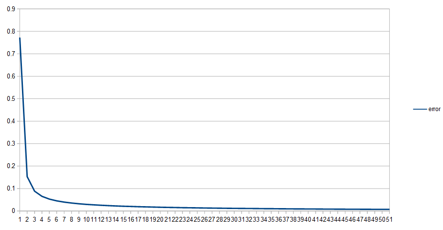
The other examples show a similarly shaped graph, where there is a lot of learning in the very beginning, and then there is a very long tail of learning very slowly.
When you train neural networks as I’ve described them, you will almost always see this, and sometimes will also see a slow learning time at the BEGINNING of the training.
This issue is also due to the activation function used, just like the unstable gradient problem, and is also an active area of research.
To help fix this issue, there is something called a “cross entropy cost function” which you can use instead of the mean squared error cost function I have been using.
That cost function essentially cancels out the non linearity of the activation function so that you get nicer linear learning progress, and can get networks to learn more quickly and evenly. However, it only cancels out the non linearity for the LAST layer in the network. This means it’s still a problem for networks that have more layers.
Lastly, there is an entirely different thing you can use backpropagation for. We adjusted the weights and biases to get our desired output for the desired inputs. What if instead we adjusted our inputs to give us the desired outputs?
You can do that by using backpropagation to calculate the dCost/dInput derivatives and using those to adjust the input, in the exact same way we adjusted the weights and biases.
You can use this to do some interesting things, including:
- finding images that a network will recognize as a familiar object, that a human wouldn’t. Start with static as input to the network, and adjust inputs to give the desired output.
- Modifying images that a network recognizes, into images it doesn’t recognize, but a human would. Start with a well recognized image, and adjust inputs using gradient ASCENT (add the derivatives, don’t subtract them) until the network stops recognizing it.
Believe it or not, this is how all those creepy “deep dream” images were made that came out of google as well, like the one below.

Now that you know the basics, you are ready to learn some more if you are interested. If you still have some questions about things I did or didn’t talk about, these resources might help you make sense of it too. I used these resources and they were all very helpful! You can also give me a shout in the comments below, or on twitter at @Atrix256.
A Step by Step Backpropagation Example
Neural Networks and Deep Learning
Backpropogation is Just Steepest Descent with Automatic Differentiation
Chain Rule
Deep Vis


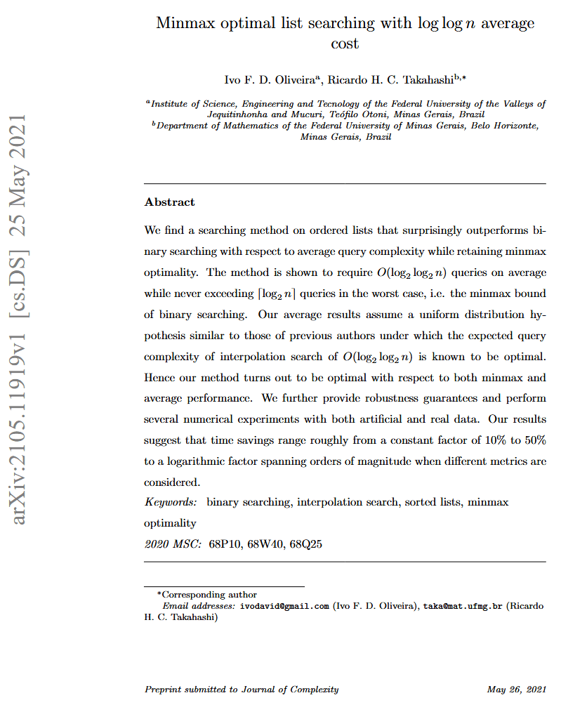


 is the sum of all the values in the rectangle from
  to
to  inclusively, but what if we want to find the sum of a different rectangle? What if we have 4 points A,B,C,D and we want to know the sum of the numbers within that sub-rectangle?


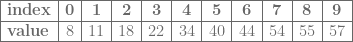
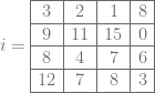
 more bits of storage which means we would need 2 more bits of storage in this case for the 2×2 grid (4 samples), making it be 5 bits total per value (3 bits of storage + 2 extra bits to hold the sum of 4 values). That would let us store the proper table:
 is 0.
is 0. is 2.
is 2. , it takes one input so is one dimensional.
 which we are still going to call one dimensional, despite it now having two dimensions.
 or
or  ) and b is where the line crosses the y axis.
 (which puts you at
  ), and let’s say that you want to go downhill from where you were at. You could do that by looking at the slope / derivative at that point, which is 3 (it’s 3 for every point on the line). Since the derivative is positive, that means going to the right will make the y value larger (you’ll go up hill) and going to the left will make the y value smaller (you’ll go down hill).
 ?
?
 . Now, which way do you move to go downhill?
 , which you can plug your x value into to get the slope / derivative at that point: -2.
 , and let’s say that we want to go down hill. Instead of just having one variable to take the derivative of (x), we now have two variables (x and y). How are we going to deal with this?


 which looks like this:
 which ended up working better for me:


 – “mu” is the mean. This is the average value of the distribution. This is where the center (peak) of the curve is on the x axis.
 – “sigma squared” is the variance, and is just the standard deviation squared. I find standard deviation more intuitive to think about.
 – “sigma” is the standard deviation, which (surprise surprise!) is the square root of the variance. This controls the “width” of the graph. The area under the cover is 1.0, so as you increase standard deviation and make the graph wider, it also gets shorter.
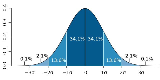
 . Note that if you instead are generating random numbers in [1,N], the mean instead is
  .
. . The standard deviation is the square root of that.
 steps, where
  is the number of items in the list. In this post’s solution, it always takes
  steps.
 ,
,  ,
,  , etc (where B is the base), you instead treat them as
  ,
,  ,
,  and so on. In other words, you multiply each digit by a fraction and add up the results.
 , so we can see that 110 is in fact 6 in binary.
 .
. .
.


