June « 2022 « The blog at the bottom of the sea

This post will first talk about how to do equality constraints in least squares curve fitting before showing how to fit multiple piecewise curves to a single set of data. The equality constraints will be used to be able to make the curves c0 continuous, c1 continuous, or higher continuity, as desired.

Point Constraints

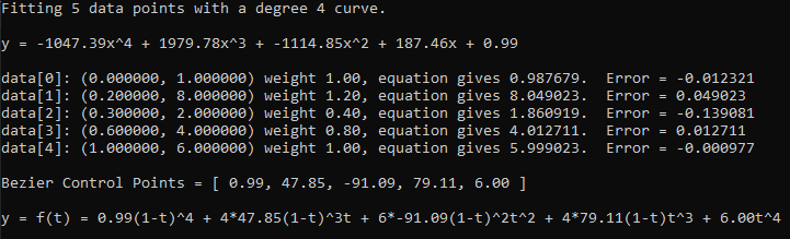
The previous blog post (https://blog.demofox.org/2022/06/06/fitting-data-points-with-weighted-least-squares/) showed how to give weights to points that were fit with least squares. If you want a curve to pass through a specific point, you could add it to the list of points to fit to, but give it a very large weighting compared to the other points, such as a weight of 1000, when the others have a weight of 1.

There is a more direct way to force a curve to go through a point though. I’ll link to some resources giving the derivation details at the end of the post, but for now I’ll just show how to do it.

For ordinary least squares, when making the augmented matrix to solve the system of linear equations it looks like this:

$\begin{bmatrix}A^TA|A^TY\end{bmatrix}$

You can use Gauss Jordan Elimination to solve it for instance (more on that here: https://blog.demofox.org/2017/04/10/solving-n-equations-and-n-unknowns-the-fine-print-gauss-jordan-elimination/)

Doing that solves for c in the equation below, where c is the vector of coefficients of the polynomial that minimizes the sum of squared error for all of the points.

$A^TA*c = A^TY$

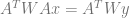
For weighted least squares it became this:

$\begin{bmatrix}A^TWA|A^TWY\end{bmatrix}$

Which again solves for c in the equation below:

$A^TWA*c = A^TWY$

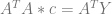
If you want to add an equality constraint to this, you make a vector C and a scalar value Z. The vector C is the values you multiply the polynomial coefficients by, and Z is the value you want to get out when you do that multiplication. You can add multiple rows, so C can be a matrix, but it needs to have as many columns as the $A^TA$ matrix does. Z then becomes a vector, which should have as many rows as the C matrix does. The matrix to solve then becomes:

$\left[\begin{array}{rr|r} A^TWA & C^T & A^TWY \\ C & 0 & Z \end{array}\right]$

When solving that and getting the coefficients out, you can ignore the extra values on the right where $Z$ is; those are the values of the Lagrange multipliers (see derivation for more details). It’s just the values where $A^TWY$ is, that become the polynomial coefficients.

Let’s see an example of a point constraint for a linear equation.

A linear equation is $y=ax+b$ where a and b are the coefficients that we are solving for.

in our case, our equation is more generalized into 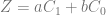$Z = aC_1 + bC_0$ where our constraint specifies $Z$ , $C_0$ and $C_1$ .

To make a point constraint, we set $C_0$ to be 1 (aka x value to the 0th power), and we set $C_1$ to be the x value (aka x value to the 1st power). We are making the powers of x for our point just like we do when making the $A$ matrix. Our Z value is the y value we want at that x location.

So, more specifically, if we wanted a linear fit to pass through the point (2, 4), our C vector would be $[1, 2]$ and our Z value would be 4.

If we wanted to give the same point constraint to a quadratic function, the C vector would be $[1, 2, 4]$ and the Z value would still be 4.

For a cubic, the C vector would be $[1, 2, 4, 8]$ and the Z value would still be 4.

If you wanted to constrain a quadratic function to 2 specific points (2,4) and (3, 2), C would become a matrix and would be:

$\begin{bmatrix}1 & 2 & 4 \\ 1 & 3 & 9\end{bmatrix}$

Z would become a vector and would be $\begin{bmatrix} 4 \\ 2\end{bmatrix}$ .

Hopefully makes sense.

There are limitations on the constraints you can give, based on the hard limitations of mathematics. For instance, you can’t tell a linear fit that it has to pass through 3 non colinear points.

Point Constraints vs Weights

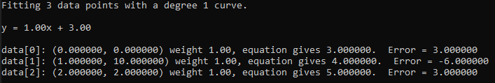
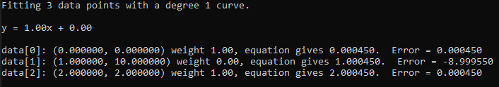
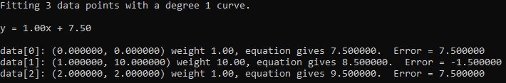
Let’s see how weights work versus constraints. First in a linear equation where we fit a line to two points, and have a third point that starts off with a weight of 0, then goes to 1, 2, 4, and then 100. Finally we’ll show what the fit looks like with an actual constraint, instead of just a weighted point.

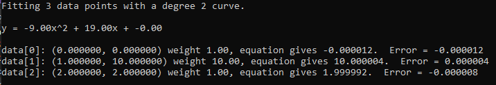
Here is the same with a quadratic curve.

The constraints let you say “This must be true” and then it does a least squares error solve for the points being fit, without violating the specified constraint. As the weight of a point becomes larger, it approaches the same effect that a constraint gives.

Derivative Constraint

A nice thing about how constraints are specified is that they aren’t limited to point constraints. You are just giving values (Z) that you want when multiplying the unknown polynomial coefficients by known values (C).

If we take the derivative of a quadratic function $y=ax^2+bx+c$ , we get $y'=2ax+b$ .

We can use this to specify that we want a specific derivative value at a specific x location. We plug the derivative we want in as the Z value, and our C constraint vector becomes $[0, 1, 2x]$ . So, if we wanted our quadratic curve to have a slope of 5 at x=1, then our Z value is 5, and our C constraint vector becomes $[0, 1, 2]$ . Below is an image which has 3 points to fit with a quadratic curve, but also has this exact slope constraint:

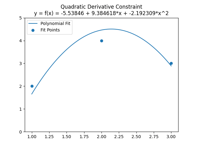
You can check the equation to verify that when x is 1, it has a slope of 5. Plugging in the coefficients and the value of 1 for x, you get 9.384618 + 2 * -2.192309 = 5.

It made sure the slope at x=1 is 5, and then did a quadratic curve fit to the points without violating that constraint, to find the minimal sum of squared errors. Pretty cool!

Piecewise Curves Without Constraints

Next, let’s see how to solve multiple piecewise curves at a time.

The first thing you do is break the data you want to fit up along the x axis into multiple groups. Each group will be fit by a curve independently, as if you did an independent curve fit for each group independently. We’ll put them all into one matrix though so that later on we can use constraints to make them connect to each other.

Let’s say that we have 6 points (1,3), (2,4), (3,2), (4, 6), (5,7), (6,5), and that we want to fit them with two linear curves. The first curve will fit the data points where x <= 3, and the second curve will fit the data points where x > 3. If we did that as described, there’d be a gap between the 3rd and 4th point though, so we’ll duplicate the (3,2) point, so that it can be the end of the first curve, and the start of the second curve.

For handling multiple curves, we change what is in the A matrix. Normally for a linear fit of 7 points, this matrix would be 2 columns and 7 rows. The first column would be x^0 for each data point, and the second column would be x^1 for each data point. Since we want to fit two linear curves to these 7 data points, our A matrix is instead going to be 4 columns (2 times the number of curves we want to fit) by 7 rows (the number of data points). The first 3 points use the first two columns, and the last four points use the second two columns, like this:

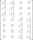
$\begin{bmatrix}x_0^0 & x_0^1 & 0 & 0 \\ x_1^0 & x_1^1 & 0 & 0 \\ x_2^0 & x_2^1 & 0 & 0 \\ 0 & 0 & x_3^0 & x_3^1 \\ 0 & 0 & x_4^0 & x_4^1 \\ 0 & 0 & x_5^0 & x_5^1 \\ 0 & 0 & x_6^0 & x_6^1 \end{bmatrix}$

When we plug in the x values for our points we get:

$A = \begin{bmatrix}1 & 1 & 0 & 0 \\ 1 & 2 & 0 & 0 \\ 1 & 3 & 0 & 0 \\ 0 & 0 & 1 & 3 \\ 0 & 0 & 1 & 4 \\ 0 & 0 & 1 & 5 \\ 0 & 0 & 1 & 6 \end{bmatrix}$

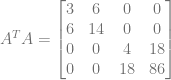
Multiplying that A matrix by it’s transpose to get $A^TA$ , we get:

$A^TA = \begin{bmatrix} 3 & 6 & 0 & 0 \\ 6 & 14 & 0 & 0 \\ 0 & 0 & 4 & 18 \\ 0 & 0 & 18 & 86 \end{bmatrix}$

Multiplying the A matrix transposed by the y values of our points, we get:

$A^TY = \begin{bmatrix} 9 \\ 17 \\ 20 \\ 95 \end{bmatrix}$

Making that into an augmented matrix of $[A^TA | A^TY]$ and then solving, we get coefficients of:

$\begin{bmatrix} 4 \\ -1/2 \\ 1/2 \\ 1 \end{bmatrix}$ .

The top two coefficients are for the points where x <= 3, and the bottom two coefficients are for the points where x > 3.

$y=-1/2x+4$ (when x <= 3)

$y= x+1/2$ (when x > 3)

Piecewise Curves With Constraints

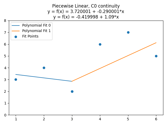
If we wanted those lines to touch at x=3 instead of being disjoint, we can do that with a constraint!

First remember we are solving for two sets of linear equation coefficients, which we’ll call $c_a$ and $c_b$ , each being a vector of the two coefficients needed by our linear equation. If we set the two linear equations equal to each other, we get this:

$c_{a1} * x + c_{a0} = c_{b1} * x + c_{b0}$

now we plug in 3 for x, and we’ll add an explicit multiplication by 1 to the constant terms:

$c_{a1} * 3 + c_{a0} * 1 = c_{b1} * 3 + c_{b0} * 1$

Now we move the right side equation over to the left side:

$c_{a1} * 3 + c_{a0} * 1 + c_{b1} * -3 + c_{b0} * -1 = 0$

We can now turn this into a constraint vector C and a value Z! When making the C vector, keep in mind that it goes constant term, then x1 term for the first curve, then constant term, then x1 term for the second curve. That gives us:

$C = [1, 3, -1, -3]$

$Z = 0$

This constraint says “I don’t care what the value of Y is when X is 3, but they should be equal to each other in both linear curves we are fitting”.

Even though the contents of our A matrix changed, the formulation for including equality constraints remains the same:

$\left[\begin{array}{rr|r} A^TWA & C^T & A^TWY \\ C & 0 & Z \end{array}\right]$

If you plug this in and solve it, you get this:

We can take this farther, and make it so the derivative at x=3 also has to match to make it C1 continuous. For a line with an equation of $y=c_1*x+c_0$ , the derivative is just $y' = c_1$ so our constraint is:

$c_{a1} = c_{b1}$

$c_{a1} - c_{b1} = 0$

As a constraint vector, this gives us:

$C = [0, 1, 0, -1]$

$Z = 0$

If we put both constraints in… that the y value must match at x=3 and also that the slope must match at x=3, we get this, which isn’t very interesting:

Since you can define a linear function as a point on the line and a slope, and we have a “must do this” constraint on both a specific point (y matches when x=3) and a slope (the slopes of the lines need to match), it came up with the same line for both parts. We’ve jumped through a lot of extra hoops to fit a single line to our data points. (Note that it is possible to say the slopes need to match and don’t say anything about the lines needing to have a matching y value. You’d get two parallel lines that fit their data points as well as they could, and would not be touching).

This gets more interesting though if we do a higher degree fit. let’s first fit the data points with two quadratic functions, with no continuity constraints. It looks like they are already C0 continuous, by random chance of the points I’ve picked, but they aren’t. Equation 1 gives y=1.999998 for x=3, while equation 2 gives 2.000089. They are remarkably close, but they are not equal.

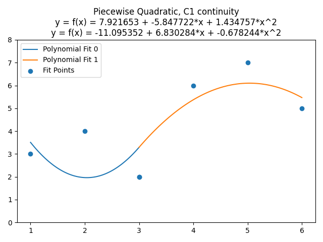
Changing it to be C0 continuous doesn’t really change it very much, so let’s skip straight to C1 continuity (which also has the C0 constraint). Remembering that the derivative of a quadratic $y=ax^2+bx+c$ , is $y'=2ax+b$ , we can set the derivatives equal to each other and plug in x for 3.

$2 * c_{a2} * x + 1 * c_{a1} = 2 * c_{b2} * x + 1 * c_{b1}$

$2 * c_{a2} * x + 1 * c_{a1} - 2 * c_{b2} * x - 1 * c_{b1} = 0$

$6 * c_{a2} + 1 * c_{a1} - 6 * c_{b2} - 1 * c_{b1} = 0$

That makes our constraint be:

$C = [0, 1, 6, 0, -1, -6]$

$Z = 0$

Plugging that in and solving, we get this very tasty fit, where the quadratic curves are C1 continuous at x=3, but otherwise are optimized to minimize the sum of the squared error of the data points:

An Oddity

I wanted to take OLS to a non matrix algebra form to see if I could get any better intuition for why it worked.

What I did was plug the symbols into the augmented matrix, did Gauss Jordan elimination with the symbols, and then looked at the resulting equations to see if they made any sense from that perspective.

Well, when doing a constant function fit like $y=a$ , a ends up being the sum of the y values, divided by the sum of the x values raised to the 0th power.

$a = \frac{\sum{y_i}}{\sum{x_i^0}}$

This makes a lot of sense intuitively, since the sum of x values to the 0th power is just the number of points of data. That makes $a$ be the average y value, or the expected y value. That checks out and makes a lot of sense.

Moving onto a linear fit $y=c_1 x + c_0$ , the $c_1$ term is calculated as:

$c_1 = \frac{\sum{(x_i y_i)} \sum{x_i^0} - \sum{x_i} \sum{y_i}}{\sum{(x_i x_i)} \sum{x_i^0} - \sum{x_i} \sum{x_i}}$

What’s strange about this formula, is that it ALMOST looks like the covariance of x and y, divided by the covariance of x and x (aka the variance of x). Which, that kinda does look like a slope / derivative: rise over run. It isn’t exactly covariance though, which divides by the number of points to get EXPECTED values, instead of sums.

Then, the $c_0$ term is calculated as this:

$c_0 = \mathbb{E}(y) - \mathbb{E}(x) * c_1$

It again ALMOST makes sense to me, in that we have the expected value of y for the constant term, like we did in the constant function, but then we need to account for the $c_1$ term, so we multiply it by the expected x value and subtract it out.

This almost makes sense but not quite. I don’t think taking it up to quadratic would make it make more sense at this point, so I left it at that.

If you have any insights or intuition, I’d love to hear them! (hit me up at https://twitter.com/Atrix256)

Closing

The simple standalone C++ code that goes with this post, which made all the data for the graphs, and the python script that graphed them, can be found at https://github.com/Atrix256/PiecewiseLeastSquares.

A nice, more formal description of constrained least squares can be found at http://www.seas.ucla.edu/~vandenbe/133A/lectures/cls.pdf.

Here is another nice one by https://twitter.com/sandwichmaker : https://demofox2.files.wordpress.com/2022/06/constrained_point_fitting.pdf

Here is a nice read about how to determine where to put the breaks of piecewise fits, and how many breaks to make: https://towardsdatascience.com/piecewise-linear-regression-model-what-is-it-and-when-can-we-use-it-93286cfee452

Thanks for reading!

About 6 years ago I wrote about how to fit curves, surfaces, volumes, and hypervolumes to data points in an “online algorithm” version of least squares – that is, you could update the fit as new data points come in.

Incremental Least Squares Curve Fitting

Incremental Least Squares Surface and Hyper-Volume Fitting

In this post, I’m going to show how to adjust the least squares equations to be able to give weights for how important data points are in the fit. We’ll be looking at curves only, and not focusing on the “online algorithm” aspect, but this will work for both surfaces/volumes as well as the online updating.

The simple standalone C++ code that goes with this post can be found at https://github.com/Atrix256/WeightedLeastSquares

If you google weighted least squares, or look for it on youtube, almost every example you are likely to find talks about it being used when the variance of data points are different in different parts of the graph, and that is used to make points contribute more or less to the final fit.

That is a pretty neat usage case, but if you are just trying to fit a curve to data points as a way to compress data or optimize calculations, you probably are not really concerned with the variance of the data points you are trying to fit. Luckily, weighting data points in least squares is pretty simple.

Here is the equation you solve in ordinary least squares (OLS):

$A^TAx = A^Ty$

where A is a matrix that contains all the powers of x of each data point, y is a vector that contains the y values of each data point, and x is polynomial coefficients that we are trying to solve for.

A pretty straightforward way to solve this equation for x is to make an augmented matrix where the left side is $A^TA$ , and the right side is $A^Ty$ .

$\left[\begin{array}{r|r} A^TA & A^Ty \end{array}\right]$

From there you can do Gauss-Jordan elimination to solve for x (https://blog.demofox.org/2017/04/10/solving-n-equations-and-n-unknowns-the-fine-print-gauss-jordan-elimination/). At the end, the left side matrix will be the identity matrix, and the right side vector will be the value for x.

$\left[\begin{array}{r|r} I & x \end{array}\right]$

Adjusting this formula for weighting involves introducing a weight matrix called W. W has a zero in every element, except along the main diagonal where the weights of each data point are. $W_{ii} = \text{weight}_i$ .

There is something called “generalized least squares” (GLS) where the weight matrix is a covariance matrix, allowing more complex correlations to be expressed with non zeroes off of the main diagonal, but for weighted least squares, the main diagonal gets the weights of the data points.

The equation to solve for weighted least squares (WLS) becomes this:

$A^TWAx = A^TWy$

You can make an augmented matrix like before:

$\left[\begin{array}{r|r} A^TWA & A^TWy \end{array}\right]$

And use Gauss-Jordan elimination again to solve for x:

$\left[\begin{array}{r|r} I & x \end{array}\right]$

Examples

Here are a few runs of the program which again is at https://github.com/Atrix256/WeightedLeastSquares

Starting with 3 data points (0,0) (1,10), (2,2) all with the same weighting, we fit them with a line and get $y = x+3$ . It’s interesting to see that data points 0 and 2 each have an error of +3 while data point 1 has an error of -6.

If we set the weighting of the 2nd point to 0.0001, we can see that it absorbs most of the error, because the weighting says that it is 10,000 times less important than the other data points.

Alternately, we can give it a weight of 10.0 to make it ten times as important as the other two data points. The error becomes a lot smaller for that data point due to it being more important.

If we switch to a quadratic curve, all three points can be well fit, with the same weights.

The example code works in any degree and also shows how to convert from these power basis polynomials to Bernstein basis polynomials, which are otherwise known as Bezier curve control points (more info on that here: https://blog.demofox.org/2016/12/08/evaluating-polynomials-with-the-gpu-texture-sampler/). The weighting you see in curves is not the same as the weighting here. When you convert the polynomial to a Bezier curve, it’s an unweighted curve. Weighted Bezier curves are made by dividing one Bezier curve by another and are called “Rational” curves, where unweighted curves are called “Integral” curves. Rational (weighted) curves are able to express more shapes than integral curves can, even when those integral curves are made by weighted least squares.

Closing

While we used weighted least squares to give different weightings to different data points, the main motivation you find on the internet seems to be about having different levels of confidence in the data points you get. This makes me wonder if we could use this in graphics, using 1/PDF(x) as the weighting in the least squares fitting like we do in importance sampled monte carlo integration. This seems especially useful if using this as an “online algorithm” that was improving a fit as it got more samples, either spatially or temporally.

The blog at the bottom of the sea

Programming, Graphics, Gamedev, Exotic Computation, Audio Synthesis

Monthly Archives: June 2022

Piecewise Least Squares Curve Fitting

Point Constraints

Point Constraints vs Weights

Derivative Constraint

Piecewise Curves Without Constraints

Piecewise Curves With Constraints

An Oddity

Closing

Fitting Data Points With Weighted Least Squares

Examples

Closing