I recently saw some interesting posts on twitter about the normal distribution:
I’m not really a statistics kind of guy, but knowing that probability distributions come up in graphics (Like in PBR & Path Tracing), it seemed like a good time to upgrade knowledge in this area while sharing an interesting technique for generating normal distribution random numbers.
Basics
Below is an image showing a few normal (aka Gaussian) distributions (from wikipedia).
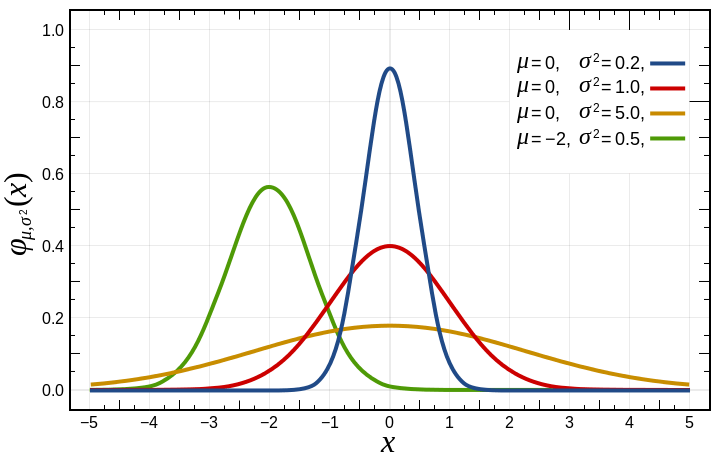
Normal distributions are defined by these parameters:
– “mu” is the mean. This is the average value of the distribution. This is where the center (peak) of the curve is on the x axis.
– “sigma squared” is the variance, and is just the standard deviation squared. I find standard deviation more intuitive to think about.
– “sigma” is the standard deviation, which (surprise surprise!) is the square root of the variance. This controls the “width” of the graph. The area under the cover is 1.0, so as you increase standard deviation and make the graph wider, it also gets shorter.
Here’s a diagram of standard deviations to help understand them (also from wikipedia):
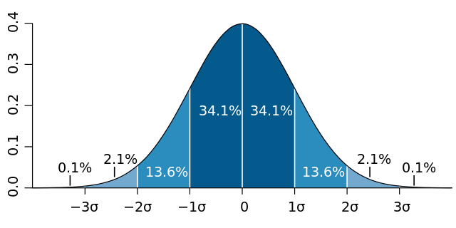
I find the standard deviation intuitive because 68.2% of the data is within one standard deviation from the mean (on the plus and minus side of the mean). 95.4% of the data is within two standard deviations of the mean.
Standard deviation is given in the same units as the data itself, so if a bell curve described scores on a test, with a mean of 80 and a standard deviation of 5, it means that 68.2% of the students got between 75 and 85 points on the test, and that 95.4% of the students got between 70 and 90 points on the test.
The normal distribution is what’s called a “probability density function” or pdf, which means that the y axis of the graph describes the likelyhood of the number on the x axis being chosen at random.
This means that if you have a normal distribution that has a specific mean and variance (standard deviation), that numbers closer to the mean are more likely to be chosen randomly, while numbers farther away are less likely. The variance controls how the probability drops off as you get farther away from the mean.
Thinking about standard deviation again, 68.2% of the random numbers generated will be within 1 standard deviation of the mean (+1 std dev or -1 std dev). 95.4% will be within 2 standard deviations.
Generating Normal Distribution Random Numbers – Coin Flips
Generating uniform random numbers, where every number is as likely as every other number, is pretty simple. In the physical world, you can roll some dice or flip some coins. In the software world, you can use PRNGs.
How would you generate random numbers that follow a normal distribution though?
In C++, there is std::normal_distribution that can do this for you. There is also something called the Box-Muller transform that can turn uniformly distributed random numbers into normal distribution random numbers (info here: Generating Gaussian Random Numbers).
I want to talk about something else though and hopefully build some better intuition.
First let’s look at coin flips.
If you flip a fair coin a million times and keep a count of how many heads and tails you saw, you might get 500014 heads and 499986 tails (I got this with a PRNG – std::mt19937). That is a pretty uniform distribution of values in the range of [0,1]. (breadcrumb: pascal’s triangle row 2 is 1,1)
Let’s flip two coins at a time though and add our values together (say that heads is 0 and tails is 1). Here’s what that graph looks like:
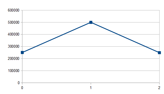
Out of 1 million flips, 250639 had no tails, 500308 had one tail, and 249053 had two tails. It might seem weird that they aren’t all even, but it makes more sense when you look at the outcome of flipping two coins: we can get heads/heads (00), heads/tails (01), tails/heads (10) or tails/tails (11). Two of the four possibilities have a single tails, so it makes sense that flipping two coins and getting one coin being a tail would be twice as likely as getting no tails or two tails. (breadcrumb: pascal’s triangle row 3 is 1,2,1)
What happens when we sum 3 coins? With a million flips I got 125113 0’s, 375763 1’s, 373905 2’s and 125219 3’s.
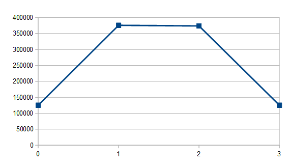
If you work out the possible combinations, there is 1 way to get 0, 3 ways to get 1, 3 ways to get 2 and 1 way to get 3. Those numbers almost exactly follow that 1, 3, 3, 1 probability. (breadcrumb: pascal’s triangle row 4 is 1,3,3,1)
If we flip 100 coins and sum them, we get this:
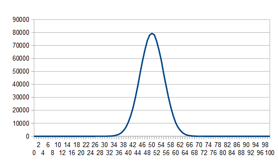
That looks a bit like the normal distribution graphs at the beginning of this post doesn’t it?
Flipping and summing coins will get you something called the “Binomial Distribution”, and the interesting thing there is that the binomial distribution approaches the normal distribution the more coins you are summing together. At an infinite number of coins, it is the normal distribution.
Generating Normal Distribution Random Numbers – Dice Rolls
What if instead of flipping coins, we roll dice?
Well, rolling a 4 sided die a million times, you get each number roughly the same percentage of the time as you’d expect; roughly 25% each. 250125 0’s, 250103 1’s, 249700 2’s, 250072 3’s.
If we sum two 4 sided dice rolls we get this:
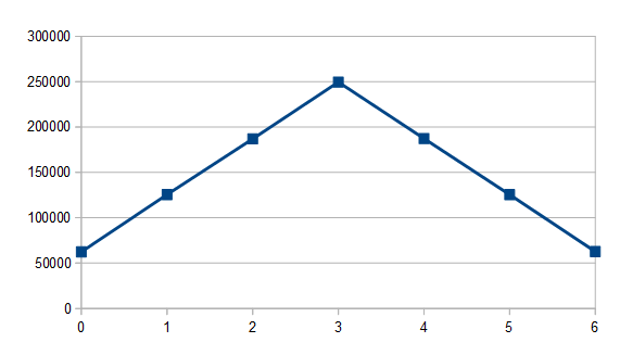
If we sum three 4 sided dice rolls we get this:
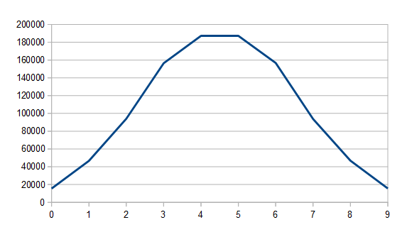
And if we sum one hundred we get this, which sure looks like a normal distribution:
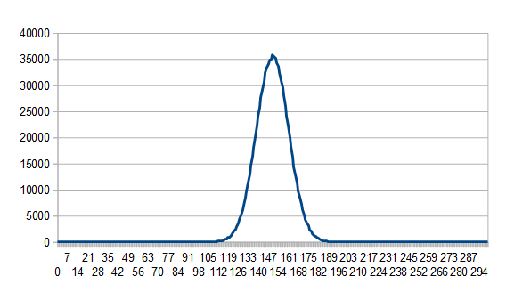
This isn’t limited to four sided dice though, here’s one hundred 6 sided dice being summed:
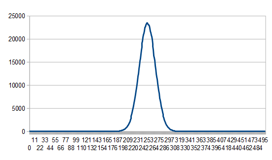
With dice, instead of being a “binomial distribution”, it’s called a “multinomial distribution”, but as the number of dice goes to infinity, it also approaches the normal distribution.
This means you can get a normal distribution with not only coins, but any sided dice in general.
An even stronger statement than that is the Central Limit Theorem which says that if you have random numbers from ANY distribution, if you add enough of em together, you’ll often approach a normal distribution.
Strange huh?
Generating Normal Distribution Random Numbers – Counting Bits
Now comes a fun way of generating random numbers which follow a normal distribution. Are you ready for it?
Simply generate an N bit random number and return how many 1 bits are set.
That gives you a random number that follows a normal distribution!
One problem with this is that you have very low “resolution” random numbers. Counting the bits of a 64 bit random number for instance, you can only return 0 through 64 so there are only 65 possible random numbers.
That is a pretty big limitation, but if you need normal distribution numbers calculated quickly and don’t mind if they are low resolution (like in a pixel shader?), this technique could work well for you.
Another problem though is that you don’t have control over the variance or the mean of the distribution.
That isn’t a super huge deal though because you can easily convert numbers from one normal distribution into another normal distribution.
To do so, you get your normal distribution random number. First you subtract the mean of the distribution to make it centered on 0 (have a mean of 0). You then divide it by the standard deviation to make it be part of a distribution which has a standard deviation of 1.
At this point you have a random number from a normal distribution which has a mean of 0 and a standard deviation of 1.
Next, you multiply the number by the standard deviation of the distribution you want, and lastly you add the mean of the distribution you want.
That’s pretty simple (and is implemented in the source code at the bottom of this post), but to do this you need to know what standard deviation (variance) and mean you are starting with.
If you have some way to generate random numbers in [0, N) and you are summing M of those numbers together, the mean is 

The variance in either case is 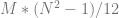
Using that information you have everything you need to generate normal distribution random numbers of a specified mean and variance.
Thanks to @fahickman for the help on calculating mean and variance of dice roll sums.
Code
Here is the source code I used to generate the data which was used to generate the graphs in this post. There is also an implementation of the bit counting algorithm i mentioned, which converts to the desired mean and variance.
#define _CRT_SECURE_NO_WARNINGS

#include <array>
#include <random>
#include <stdint.h>
#include <stdio.h>
#include <limits>

const size_t c_maxNumSamples = 1000000;
const char* c_fileName = "results.csv";

template <size_t DiceRange, size_t DiceCount, size_t NumBuckets>
void DumpBucketCountsAddRandomNumbers (size_t numSamples, const std::array<size_t, NumBuckets>& bucketCounts)
{
    // open file for append if we can
    FILE* file = fopen(c_fileName, "a+t");
    if (!file)
        return;

    // write the info
    float mean = float(DiceCount) * float(DiceRange - 1.0f) / 2.0f;
    float variance = float(DiceCount) * (DiceRange * DiceRange) / 12.0f;
    if (numSamples == 1)
    {
        fprintf(file, "\"%zu random numbers [0,%zu) added together (sum %zud%zu). %zu buckets.  Mean = %0.2f.  Variance = %0.2f.  StdDev = %0.2f.\"\n", DiceCount, DiceRange, DiceCount, DiceRange, NumBuckets, mean, variance, std::sqrt(variance));
        fprintf(file, "\"\"");
        for (size_t i = 0; i < NumBuckets; ++i)
            fprintf(file, ",\"%zu\"", i);
        fprintf(file, "\n");
    }
    fprintf(file, "\"%zu samples\",", numSamples);

    // report the samples
    for (size_t count : bucketCounts)
        fprintf(file, "\"%zu\",", count);

    fprintf(file, "\"\"\n");
    if (numSamples == c_maxNumSamples)
        fprintf(file, "\n");

    // close file
    fclose(file);
}

template <size_t DiceSides, size_t DiceCount>
void AddRandomNumbersTest ()
{
    std::mt19937 rng;
    rng.seed(std::random_device()());
    std::uniform_int_distribution<size_t> dist(size_t(0), DiceSides - 1);

    std::array<size_t, (DiceSides - 1) * DiceCount + 1> bucketCounts = { 0 };

    size_t nextDump = 1;
    for (size_t i = 0; i < c_maxNumSamples; ++i)
    {
        size_t sum = 0;
        for (size_t j = 0; j < DiceCount; ++j)
            sum += dist(rng);

        bucketCounts[sum]++;

        if (i + 1 == nextDump)
        {
            DumpBucketCountsAddRandomNumbers<DiceSides, DiceCount>(nextDump, bucketCounts);
            nextDump *= 10;
        }
    }
}

template <size_t NumBuckets>
void DumpBucketCountsCountBits (size_t numSamples, const std::array<size_t, NumBuckets>& bucketCounts)
{
    // open file for append if we can
    FILE* file = fopen(c_fileName, "a+t");
    if (!file)
        return;

    // write the info
    float mean = float(NumBuckets-1) * 1.0f / 2.0f;
    float variance = float(NumBuckets-1) * 3.0f / 12.0f;
    if (numSamples == 1)
    {
        fprintf(file, "\"%zu random bits (coin flips) added together. %zu buckets.  Mean = %0.2f.  Variance = %0.2f.  StdDev = %0.2f.\"\n", NumBuckets - 1, NumBuckets, mean, variance, std::sqrt(variance));
        fprintf(file, "\"\"");
        for (size_t i = 0; i < NumBuckets; ++i)
            fprintf(file, ",\"%zu\"", i);
        fprintf(file, "\n");
    }
    fprintf(file, "\"%zu samples\",", numSamples);

    // report the samples
    for (size_t count : bucketCounts)
        fprintf(file, "\"%zu\",", count);

    fprintf(file, "\"\"\n");
    if (numSamples == c_maxNumSamples)
        fprintf(file, "\n");

    // close file
    fclose(file);
}

template <size_t NumBits> // aka NumCoinFlips!
void CountBitsTest ()
{

    size_t maxValue = 0;
    for (size_t i = 0; i < NumBits; ++i)
        maxValue = (maxValue << 1) | 1;

    std::mt19937 rng;
    rng.seed(std::random_device()());
    std::uniform_int_distribution<size_t> dist(0, maxValue);

    std::array<size_t, NumBits + 1> bucketCounts = { 0 };

    size_t nextDump = 1;
    for (size_t i = 0; i < c_maxNumSamples; ++i)
    {
        size_t sum = 0;
        size_t number = dist(rng);
        while (number)
        {
            if (number & 1)
                ++sum;
            number = number >> 1;
        }

        bucketCounts[sum]++;

        if (i + 1 == nextDump)
        {
            DumpBucketCountsCountBits(nextDump, bucketCounts);
            nextDump *= 10;
        }
    }
}

float GenerateNormalRandomNumber (float mean, float variance)
{
    static std::mt19937 rng;
    static std::uniform_int_distribution<uint64_t> dist(0, (uint64_t)-1);

    static bool seeded = false;
    if (!seeded)
    {
        seeded = true;
        rng.seed(std::random_device()());
    }

    // generate our normal distributed random number from 0 to 65.
    //
    float sum = 0.0f;
    uint64_t number = dist(rng);
    while (number)
    {
        if (number & 1)
            sum += 1.0f;
        number = number >> 1;
    }

    // convert from: mean 32, variance 16, stddev 4
    // to: mean 0, variance 1, stddev 1
    float ret = sum;
    ret -= 32.0f;
    ret /= 4.0f;

    // convert to the specified mean and variance
    ret *= std::sqrt(variance);
    ret += mean;
    return ret;
}

void VerifyGenerateNormalRandomNumber (float mean, float variance)
{
    // open file for append if we can
    FILE* file = fopen(c_fileName, "a+t");
    if (!file)
        return;

    // write info
    fprintf(file, "\"Normal Distributed Random Numbers. mean = %0.2f.  variance = %0.2f.  stddev = %0.2f\"\n", mean, variance, std::sqrt(variance));

    // write some random numbers
    fprintf(file, "\"100 numbers\"");
    for (size_t i = 0; i < 100; ++i)
        fprintf(file, ",\"%f\"", GenerateNormalRandomNumber(mean, variance));
    fprintf(file, "\n\n");

    // close file
    fclose(file);
}

int main (int argc, char **argv)
{
    // clear out the file
    FILE* file = fopen(c_fileName, "w+t");
    if (file)
        fclose(file);

    // coin flips
    {
        // flip a fair coin
        AddRandomNumbersTest<2, 1>();

        // flip two coins and sum them
        AddRandomNumbersTest<2, 2>();

        // sum 3 coin flips
        AddRandomNumbersTest<2, 3>();

        // sum 100 coin flips
        AddRandomNumbersTest<2, 100>();
    }

    // dice rolls
    {
        // roll a 4 sided die
        AddRandomNumbersTest<4, 1>();

        // sum two 4 sided dice
        AddRandomNumbersTest<4, 2>();

        // sum three 4 sided dice
        AddRandomNumbersTest<4, 3>();

        // sum one hundred 4 sided dice
        AddRandomNumbersTest<4, 100>();

        // sum one hundred 6 sided dice
        AddRandomNumbersTest<6, 100>();
    }

    CountBitsTest<8>();
    CountBitsTest<16>();
    CountBitsTest<32>();
    CountBitsTest<64>();

    VerifyGenerateNormalRandomNumber(0.0f, 20.0f);

    VerifyGenerateNormalRandomNumber(0.0f, 10.0f);

    VerifyGenerateNormalRandomNumber(5.0f, 10.0f);

    return 0;
}