Dissecting “Tiny Clouds”

There is an amazing shadertoy called “Tiny Clouds” by stubbe (twitter: @Stubbesaurus) which flies you through nearly photorealistic clouds in only 10 lines of code / 280 characters (2 old sized tweets or 1 new larger sized tweet).

The code is a bit dense, so I wanted to take some time to understand it and share the explanation for anyone else who was interested. Rune (the author) kindly answered a couple questions for me as well. Thanks Rune!

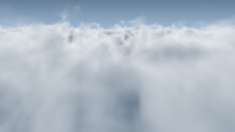
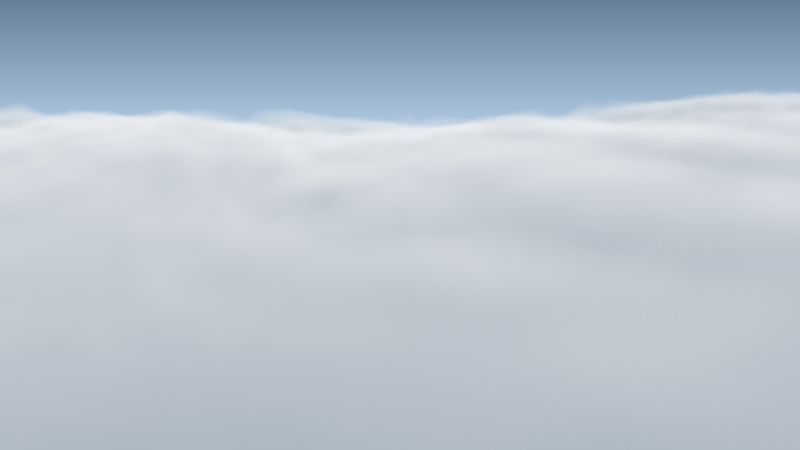
Link: [SH17A] Tiny Clouds (Check out this link, it looks even more amazing in motion)

Here is the code in full. The texture in iChannel0 is just a white noise texture that is bilinearly sampled.

#define T texture(iChannel0,(s*p.zw+ceil(s*p.x))/2e2).y/(s+=s)*4.
void mainImage(out vec4 O,vec2 x){
    vec4 p,d=vec4(.8,0,x/iResolution.y-.8),c=vec4(.6,.7,d);
    O=c-d.w;
    for(float f,s,t=2e2+sin(dot(x,x));--t>0.;p=.05*t*d)
        p.xz+=iTime,
        s=2.,
        f=p.w+1.-T-T-T-T,
    	f<0.?O+=(O-1.-f*c.zyxw)*f*.4:O;
}

BTW this shadertoy is a shrunken & reinterpreted version of a larger, more feature rich shadertoy by iq: Clouds

Before diving into the details of the code, here is how it works in short:

  • Every pixel does a ray march from far to near. It does it backwards to make for simpler alpha blending math.
  • At every ray step, it samples FBM data (fractal brownian motion) to figure out if the current position is below the surface of the cloud or above it.
  • If below, it alpha blends the pixel color with the cloud color at that point, using the vertical distance into the cloud as the cloud density.

Pretty reasonable and simple – and it would have to be, to look so good in so few characters! Let’s dig into the code.

#define T texture(iChannel0,(s*p.zw+ceil(s*p.x))/2e2).y/(s+=s)*4.
void mainImage(out vec4 O,vec2 x){
    vec4 p,d=vec4(.8,0,x/iResolution.y-.8),c=vec4(.6,.7,d);
    O=c-d.w;
    for(float f,s,t=2e2+sin(dot(x,x));--t>0.;p=.05*t*d)
        p.xz+=iTime,
        s=2.,
        f=p.w+1.-T-T-T-T,
    	f<0.?O+=(O-1.-f*c.zyxw)*f*.4:O;
}

Line 1 is a define that we’ll come back to and line 2 is just a minimal definition of the mainImage function.

#define T texture(iChannel0,(s*p.zw+ceil(s*p.x))/2e2).y/(s+=s)*4.
void mainImage(out vec4 O,vec2 x){
    vec4 p,d=vec4(.8,0,x/iResolution.y-.8),c=vec4(.6,.7,d);
    O=c-d.w;
    for(float f,s,t=2e2+sin(dot(x,x));--t>0.;p=.05*t*d)
        p.xz+=iTime,
        s=2.,
        f=p.w+1.-T-T-T-T,
    	f<0.?O+=(O-1.-f*c.zyxw)*f*.4:O;
}

On line 3 several variables are declared:

  • p – this is the variable that holds the position of the ray during the ray march. It isn’t initialized here, but that’s ok because the position is calculated each step in the loop. It is interesting to see that the y component of p is never used. p.x is actually depth into the screen, p.z is the screen x axis, and p.w is the screen y axis (aka the up axis). I believe that the axis choices and the fact that the y component is never used is purely to make the code smaller.
  • d – this is the direction that the ray for this pixel travels in. It uses the same axis conventions as p, and the y component is also never used (except implicitly for calculating p.y, which is never used). 0.8 is subtracted from d.z and d.w (the screen x and screen y axes). Interestingly that makes the screen x axis 0 nearly centered on the screen. It also points the screen y axis downward a bit, putting the 0 value near the top of the screen to make the camera look more downward at the clouds.
  • c – this is the color of the sky, which is a nice sky blue. It’s initialized with constants in x and y, and then d is used for z and w. d.xy goes into c.zw. That gives c the 0.8 value in the z field. I’m sure it was done this way because it’s fewer characters to initialize using “d” compared to “.8,0.” for the same effect. Note that c.w is used to calculate O.w (O.a) but that the alpha channel of the output pixel value is currently ignored by shadertoy, so this is a meaningless by product of the code, not a desired feature.
#define T texture(iChannel0,(s*p.zw+ceil(s*p.x))/2e2).y/(s+=s)*4.
void mainImage(out vec4 O,vec2 x){
    vec4 p,d=vec4(.8,0,x/iResolution.y-.8),c=vec4(.6,.7,d);
    O=c-d.w;
    for(float f,s,t=2e2+sin(dot(x,x));--t>0.;p=.05*t*d)
        p.xz+=iTime,
        s=2.,
        f=p.w+1.-T-T-T-T,
    	f<0.?O+=(O-1.-f*c.zyxw)*f*.4:O;
}

Line 4 initializes the output pixel color to be the sky color (c), but then subtracts d.w which is the pixel’s ray march direction on the screen y axis. This has a nice effect of making a nice sky blue gradient.

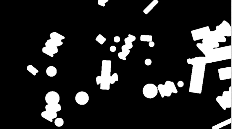
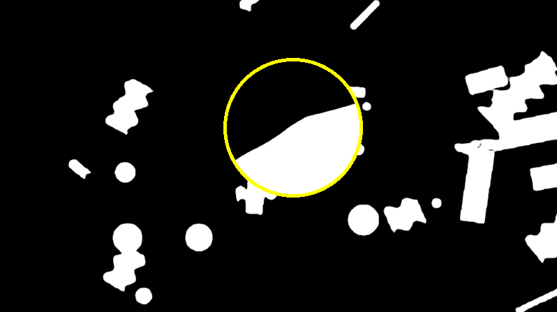
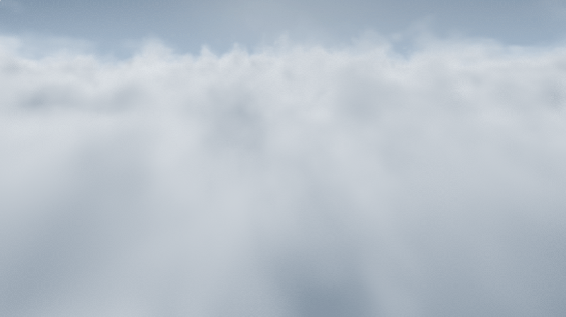
To see this in action, here we set O to c:

Here we set O to c-d.w:

It gets darker blue towards the top – where d.w is positive – because a positive number is being subtracted from the sky color. The color values get smaller.

It gets lighter towards the bottom – where d.w is negative – because a negative number is being subtracted from the sky color. The color values get larger.

#define T texture(iChannel0,(s*p.zw+ceil(s*p.x))/2e2).y/(s+=s)*4.
void mainImage(out vec4 O,vec2 x){
    vec4 p,d=vec4(.8,0,x/iResolution.y-.8),c=vec4(.6,.7,d);
    O=c-d.w;
    for(float f,s,t=2e2+sin(dot(x,x));--t>0.;p=.05*t*d)
        p.xz+=iTime,
        s=2.,
        f=p.w+1.-T-T-T-T,
    	f<0.?O+=(O-1.-f*c.zyxw)*f*.4:O;
}

On line 5, the for loop for ray marching starts. A few things happen here:

  • f is declared – f is the signed vertical distance from the current point in space to the cloud. If negative, it means that the point is inside the cloud. If positive, it means that the point is outside (above) the cloud. It isn’t initialized here, but it’s calculated each iteration of the loop so that’s fine.
  • s is declared – s is a scale value for use with the FBM data. FBMs work by sampling multiple octaves of data. You scale up the position and scale down the value for each octave. s is that scale value, used for both purposes. This isn’t initialized but is calculated each frame so that’s fine.
  • t is declared and initialized – t (aka ray march step index) is initialized to 2e2 aka 200. It was done this way because “2e2” is smaller than “200.” by one character. Note that the for loop takes t from 200 to 0. The ray marching happens back to front to simplify alpha blending. The sin(dot(x,x)) part I want to talk about briefly below.
  • p is calculated – p (aka the position in the current step of the ray march) is calculated, and this happens every step of the loop. p is t (time) multiplied by the direction of the ray for this pixel, and multiplied by .05 to scale it down.

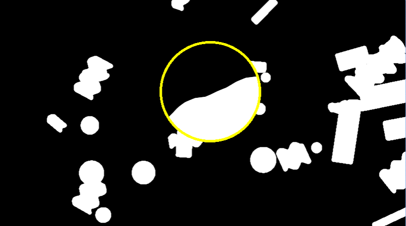
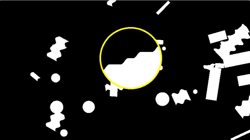
The reason that sin(dot(x,x)) is added to the “ray time” is because the ray is marching through voxelized data (boxes). Unlike boxes, clouds are supposed to look organic, and not geometric. A way to fight the problem of the data looking boxy is to add a little noise to each ray to break up the geometric pattern. You can either literally add some noise to the result, or do what this shader does, which is add some noise to the starting position of the ray so that neighboring rays will cross the box (voxel) boundaries at different times and will look noisy instead of geometric.

I can’t see a difference when removing this from the shader, and other people have said the same. Rune says in the comments that it’d be on the chopping block for sure if he needed to shave off some more characters. He reached his 280 character goal, so no there is no need to remove it.

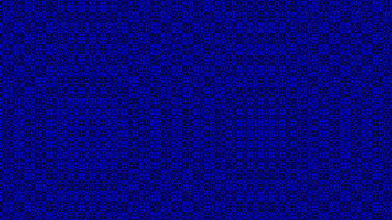
For what it’s worth, here is that expression visualized in the blue channel. the -1 to +1 is mapped to 0 to 1 by multiplying it by a half and adding a half:

#define T texture(iChannel0,(s*p.zw+ceil(s*p.x))/2e2).y/(s+=s)*4.
void mainImage(out vec4 O,vec2 x){
    vec4 p,d=vec4(.8,0,x/iResolution.y-.8),c=vec4(.6,.7,d);
    O=c-d.w;
    for(float f,s,t=2e2+sin(dot(x,x));--t>0.;p=.05*t*d)
        p.xz+=iTime,
        s=2.,
        f=p.w+1.-T-T-T-T,
    	f<0.?O+=(O-1.-f*c.zyxw)*f*.4:O;
}

Line 6 adds the current time to p.x and p.z. Remember that the x component is the axis pointing into the screen and the z component is the screen space x axis, so this line of code moves the camera forward and to the right over time.

If you are wondering why the lines in the for loop end in a comma instead of a semicolon, the reason is because if a semicolon was used instead, the for loop would require two more characters: “{” and “}” to show where the scope of the loop started and ended. Ending the lines with commas mean it’s one long statement, so the single line version of a for loop can be used. An interesting trick 😛

#define T texture(iChannel0,(s*p.zw+ceil(s*p.x))/2e2).y/(s+=s)*4.
void mainImage(out vec4 O,vec2 x){
    vec4 p,d=vec4(.8,0,x/iResolution.y-.8),c=vec4(.6,.7,d);
    O=c-d.w;
    for(float f,s,t=2e2+sin(dot(x,x));--t>0.;p=.05*t*d)
        p.xz+=iTime,
        s=2.,
        f=p.w+1.-T-T-T-T,
    	f<0.?O+=(O-1.-f*c.zyxw)*f*.4:O;
}

Line 7 sets / initializes s to 2. Remember that s is used as the octave scale for sample position and resulting value. That will come into play in the next line.

#define T texture(iChannel0,(s*p.zw+ceil(s*p.x))/2e2).y/(s+=s)*4.
void mainImage(out vec4 O,vec2 x){
    vec4 p,d=vec4(.8,0,x/iResolution.y-.8),c=vec4(.6,.7,d);
    O=c-d.w;
    for(float f,s,t=2e2+sin(dot(x,x));--t>0.;p=.05*t*d)
        p.xz+=iTime,
        s=2.,
        f=p.w+1.-T-T-T-T,
    	f<0.?O+=(O-1.-f*c.zyxw)*f*.4:O;
}

First let’s look at line 1, which is the “T” macro.

That macro samples the texture (which is just white noise) at a position described by the current ray position in the ray march. the s variable is used to scale up the position, and it’s also used to scale down the noise value at that position. The same position involves p.zw which is the screen space x and y axis respectively, but also includes p.x which is the axis pointing into the screen. This maps a 3d coordinate to a 2d texture location. I have tried making the shader sample a 3d white noise texture instead of doing this and get what looks to be the same quality results.

The macro also multiplies s by 2 each sample, so that the next sample will sample the next octave.

An interesting part of this texture coordinate conversion from 3d to 2d though is that the x component is ceil’d(the axis that goes into the screen). I’m not sure if there is any logic to this other than it’s a way to transform the 3d coordinates into a 2d one for the texture lookup.

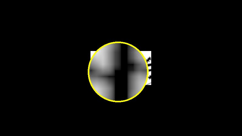
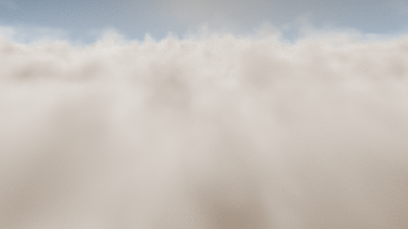
Below is what it looks like without the ceil in the macro for s*p.x. It stretches the noise in a weird way.

The uv coordinates sampled are divided by 2e2 (which is 200, but again, fewer characters than “200.”). I believe this value of 200 matches the number of ray march steps intentionally, so that the ray marches across the entire texture (with wrap around) each time.

Line 8 uses this macro. We set f to be p.w, which is the ray’s height. 1 is added to the height which moves the camera up one unit. Lastly, the T macro is used to subtract 4 octaves of noise from f.

The result of this is that f gives us a signed distance to the cloud on the vertical axis. In other words, f tells us how far above or below the surface of the clouds we are. A positive value means the position is above the clouds, and a negative value means the position is below the clouds.

#define T texture(iChannel0,(s*p.zw+ceil(s*p.x))/2e2).y/(s+=s)*4.
void mainImage(out vec4 O,vec2 x){
    vec4 p,d=vec4(.8,0,x/iResolution.y-.8),c=vec4(.6,.7,d);
    O=c-d.w;
    for(float f,s,t=2e2+sin(dot(x,x));--t>0.;p=.05*t*d)
        p.xz+=iTime,
        s=2.,
        f=p.w+1.-T-T-T-T,
    	f<0.?O+=(O-1.-f*c.zyxw)*f*.4:O;
}

Line 10 is the close of the function, so line 9 is the last meaningful line of code.

This line of code says:

  • If f less than zero (“If the point is inside the cloud”)
  • Then add “some formula” to the pixel color (more info on that in a moment)
  • Else, “O”. This is a dummy statement with no side effects that is there to satisfy the ternary operator syntax with a minimal number of characters.

I was looking at that formula for a while, trying to figure it out. I was thinking maybe it was something like a cheaper function fitting of some more complex light scattering / absorption function.

I asked Rune and he explained it. All it’s doing is doing an alpha blend (a lerp) from the current pixel color to the color of the cloud at this position. If you do the lerp mathematically, expand the function and combine terms, you get the above. Here’s his explanation from twitter (link to twitter thread):

Alpha blending between accumulated color (O) and incoming cloud color (1+f*c.zyxw). Note density (f) is negative:
O = lerp(O, 1+f*c.zyxw, -f*.4)
O = O * (1+f*.4) + (1+f*c.zyxw)*-f*.4
O = O + O*f*.4 + (1+f*c.zyxw)*-f*.4
O = O + (O-1-f*c.zyxw)*f*.4
O += (O-1-f*c.zyxw)*f*.4

Remember the marching is from far to near which simplifies the calculations quite a bit. If the marching was reversed then you would also need to keep track of an accumulated density.

One obvious question then would be: why is “1+f*c.zyxw” the cloud color of the current sample?

One thing that helps clear that up is that f is negative. if you make “f” mean “density” and flip it’s sign, the equation becomes: “1-density*c.zyxw”

We can then realize that “1” when interpreted as a vec4 is the color white, and that c is the sky color. We can also throw out the w since we (and shadertoy) don’t care about the alpha channel. We can also replace x,y,z with r,g,b. That makes the equation become: “white-density*skycolor.bgr”

In that equation, when density is 0, all we are left with is white. As density increases, the color gets darker.

The colors are the reversed sky color, because the sky color is (0.6, 0.7, 0.8). if we used the sky color instead of the reversed sky color, you can see that blue would drop away faster than green, which would drop away faster than red. If you do that, the clouds turn a reddish color like you can see here:

I’m not an expert in atmospheric rendering (check links at the bottom for more info on that!), but it looks more natural and correct for it to do the reverse. What we really want is for red to drop off the quickest, then green, then blue. I believe a more correct thing to do would be to subtract sky color from 1.0 and use that color to multiply density by. However, reversing the color channels works fine in this case, so no need to spend the extra characters!

Another obvious question might be: why is the amount of lerp “-f*.4”?

It probably looks strange to see a negative value in a lerp amount, but remembering that f is negative when it’s inside a cloud means that it’s a positive value, multiplied by 0.4 to make it smaller. It’s just scaling the density a bit.

Other Notes

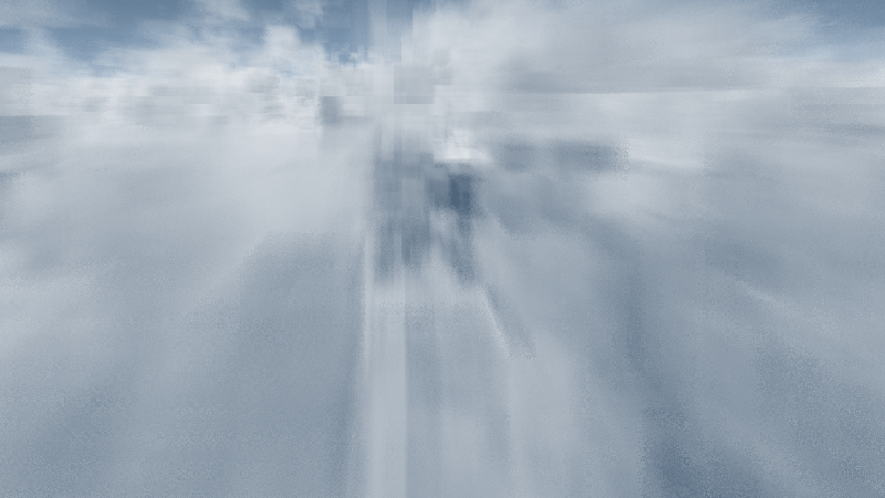
Using bilinear interpolation of the texture makes a big difference. If you switch the texture to using nearest neighbor point sampling you get something like this which looks very boxy. It looks even more boxy when it’s in motion.

One thing I wanted to try when understanding this shader was to try to replace the white noise texture lookup with a white noise function. It does indeed work as you can see below, but it got noticeably slower on my machine doing that. I’m so used to things being texture bound that getting rid of texture reads is usually a win. I didn’t stop to think that in this situation all that was happening was compute and no texture reads. In a more fully featured renderer, you may indeed find yourself texture read bound, and moving it out of a texture read could help speed things up – profile and see! It’s worth noting that to get proper results you need to discretize your noise function into a grid and use bilinear interpolation between the values – mimicing what the texture read does. Check my unpacked version of the shader in the links section for more details!

Something kind of fun is that you can replace the white noise texture with other textures. The results seem to be pretty good usually! Below is where i made the shadertoy use the “Abstract1” image as a source. The clouds got a lot more soft.

Thanks for reading. Anything that I got wrong or missed, please let me and the other readers know!

Links

Here is my unpacked version of the shader, which includes the option to use a white noise function instead of a white noise texture: Tiny Clouds: Unpacked & No Tex

Here are two great links for more information on how to render atmospheric and volumetric effects:

Volumetric Atmospheric Scattering

Creating a Volumetric Ray Marcher

Raytracing Reflection, Refraction, Fresnel, Total Internal Reflection, and Beer’s Law

This post talks about how to render images like the below in real time using ray tracing. Some realism in the images come from reflection and refraction, but the real icing on the cake comes from Fresnel, total internal reflection and Beer’s law. We’ll look at the contributions of these features individually and talk about how to properly combine them for the greatest and most realistic results (:

The renderings come from a shadertoy that accompanies this post: Shadertoy: Reflect Refract TIR Fresnel RayT

My motivation for learning more about this stuff is that I’m starting to make a marble madness inspired game, and I’m planning to do hybrid rendering between rasterization and ray based techniques.

This post will focus more on how to make these features work for you in ray tracing, and less about the reasons for why they work the way they do. This post is more about practical implementations, and less about rigorous explanations.

If you have any questions, comments, corrections or additions, feel free to leave in the comments section at the bottom, or feel free to hit me up on twitter at @Atrix256.

This post is assumes you know how to do basic raytracing with ambient, diffuse and specular lighting, like the image below, which we are going to start with:

Reflection

The first thing to talk about is reflection. More specifically we are going to be talking about SPECULAR reflection.

Specular is defined by the dictionary to mean “of, relating to, or having the properties of a mirror.”, so what we normally think of as reflection (like from a mirror) is in fact specular reflection.

There is non specular reflection, aka diffuse reflection, which just means that light is reflected off of a surface in a non mirror like way. This is accomplished with diffuse lighting where commonly we dot product the normal of a surface with the direction from the surface to the light to know how much to light that point on the surface.

If specular reflection is how mirrors reflect, and diffuse reflection is how regular diffuse surfaces work, then you might wonder what specular lighting is all about.

A specular highlight is actually just a cheap approximation to doing a mirror like specular reflection of a light source, so it is a cheap kind of specular reflection.

Let’s talk about how to do real mirror like specular reflection in a ray tracer.

When light hits a surface, some amount of the light will be reflected, and some amount of the light will be transmitted into the object. Transmitted light is used for the diffuse shading.

As you might imagine, the amount of light reflected plus the amount of light transmitted must equal the total amount of light that hit the surface. (note that some transmitted energy may be absorbed and given off as heat, or the object may be glowing, so may give off more light than received but let’s ignore that stuff for now.)

A common way to deal with this is to define a reflectivity of a surface as the amount of light it reflects in percent and use 100% minus that amount as the transmitted amount.

You might say that 2% of light that hits a surface reflects. That means that 98% of the light that hits a surface is transmitted and used for the diffuse shading.

When shading a point on the surface, you would calculate both the reflected color at that point on the surface, and the diffuse shaded color at that point, but you multiply the reflected color by 0.02 and the diffuse shaded color by 0.98 and add them together. Doing this gives a result like the below:

The higher the reflectivity percent, the more reflection you get, and the less diffuse shading you get. Turning down reflectivity has the opposite effect.

How do you calculate the reflected color of a point on a surface though?

You simply calculate the ray that reflected off of the surface, and calculate the color of what that ray hit.

To calculate a reflected ray, you need to know the direction that the ray was traveling when it hit the surface (The incident direction), you need to know the location that the ray hit the surface (the surface location), and you need to know the normal of the surface at the intersection point.

If you have those things you can calculate the reflected ray direction as this:

ReflectRayLocation = SurfaceLocation \\ ReflectRayDirection = IncidentDirection - 2 * SurfaceNormal * DotProduct(IncidentDirection, SurfaceNormal)

Note that in hlsl and glsl there is a function called “reflect” which takes the incident direction, and the surface normal, and returns you the reflected direction.

Doing the above is mathematically correct, but if you then try to raytrace from that ray, you may hit the same object you are reflecting off. One way to fight that problem is to push the ray positin a small amount away from the surface to make sure it misses it. You can do that for example like this:

ReflectRayLocation = ReflectRayLocation + ReflectRayDirection * 0.01

There are other ways to make sure you don’t hit the same object again, but pushing the ray away from the object a small amount really does work pretty nicely in practice.

Refraction

I mentioned in the last section that whatever light wasn’t reflected when it hit a surface was transmitted. I also said that the transmitted light was used for diffuse shading.

In reality, it’s passed through the “bidirectional scattering distribution function” aka BSDF. You may have heard the term “bidirectional reflection distribution function” aka BRDF. A BRDF only deals with the hemisphere (half a sphere) that surrounds the surface normal. The BSDF on the other hand deals with the full sphere surrounding a surface normal so BRDF is a subset of what is possible with the BSDF.

Because the BSDF deals with an entire sphere, that means that it can handle reflection (specular and non specular) like the BRDF can, but it can also deal with transparency and refraction, where some of the light travels THROUGH an object.

In a path tracer where everything is physically accurate and mathematically precise, we would be interested in dealing with a BSDF and integrating over the sphere, but since we are working with a ray tracer, our physical accuracy needs are a lot lower – we only want a result that looks plausible.

What we are going to do for our transparency is calculate a direction that the ray is going to travel through the object, ray trace that ray to get a color, and use the transmitted light (the portion of light that isn’t reflected) as a multiplier of that color, that we add to the reflected amount of light.

If we have an object with 10% reflectivity, and 90% transmittance, but use that transmitted light for transparency, we’ll have a rendering like below:

Now that we have transparency, let’s talk about refraction. Refraction is a physical phenomenon where light bends (“changes speed” i guess but that sounds a bit suspicious for light), as it hits a boundary between two different surfaces.

Every material has a refractive index, and in fact, may have different refractive indices per light frequency. For our purposes, we’ll assume surfaces have the same refractive index for every frequency of light. There’s a list of refractive indices for a lot of different materials here: Index of refraction

How a ray bends when it refracts depends on the ration of the refractive index that it’s leaving to the refractive index that it’s entering. AKA outside/inside.

HLSL and GLSL have a function called refract which take the incident vector, the surface normal vector, and that ration of refractive indices, and return the refracted ray.

When you do a raytrace down the refracted ray, you will have the same problem as when tracing the reflected ray, that you may hit the same surface you just hit again erroneously. To help that, you once again just move the ray slightly away from the surface.

RefractRayLocation = RefractRayLocation + RefractRayDirection * 0.01

Here is a rendering where the sphere has 10% reflectivity, 90% transmittance, an air refractive index of 1.0, and a refractive index of 1.125 for the sphere. You can see how the light bends as it goes through the object and looks pretty neat!

Fresnel

There is an interesting property in our world: If you look at something straight on, it’s the least reflective it will be. If you turn it nearly 90 degrees where it’s nearly edge on, it will be the most reflective it can be. Many surfaces will become almost perfectly reflective when you view them almost edge on. Go try it out with a wall in your house or a glass or other things.

Weird huh? That’s called Fresnel, and is something we can also make use of in ray tracing to get a more realistic image.

Instead of just always using the reflectivity amount of the surface, we use the Fresnel equation to figure out how much reflectivity an object should have based on the view angle versus the surface normal, so that when it’s more edge on it becomes more reflective. At minimum the reflectivity will be the reflectivity of the surface, and at maximum the reflectivity will be 100%.

The amount we transmit for either refraction or diffuse will be 100% minus however much percentage is reflective.

Here is the image showing normal reflection again:

Here is the image with Fresnel:

It looks quite a bit better with fresnel doesn’t it?!

Here’s a GLSL function of Schlick’s Fresnel approximation function. Notice that it takes the surface normal and incident vector, as well as the refractive index being left (n1) and the refractive index being entered (n2):

float FresnelReflectAmount (float n1, float n2, vec3 normal, vec3 incident)
{
        // Schlick aproximation
        float r0 = (n1-n2) / (n1+n2);
        r0 *= r0;
        float cosX = -dot(normal, incident);
        if (n1 > n2)
        {
            float n = n1/n2;
            float sinT2 = n*n*(1.0-cosX*cosX);
            // Total internal reflection
            if (sinT2 > 1.0)
                return 1.0;
            cosX = sqrt(1.0-sinT2);
        }
        float x = 1.0-cosX;
        float ret = r0+(1.0-r0)*x*x*x*x*x;

        // adjust reflect multiplier for object reflectivity
        ret = (OBJECT_REFLECTIVITY + (1.0-OBJECT_REFLECTIVITY) * ret);
        return ret;
}

Our tale of reflection is complete, so let’s go back to refraction / transparency and finish up the last two items.

Total Internal Reflection

The way that the Fresnel equation works, it’s possible that when moving from a material with a higher index of refraction to a lower one, that the amount of refraction can actually drop to zero percent. In this case, the light doesn’t exit the higher refractive index object and instead ONLY reflects back into the object, because the reflective amount becomes 100%.

When this happens, it’s called “Total Internal Reflection” for hopefully obvious reasons (:

There isn’t a whole lot to say about this, because you can see that this is even accounted for in the GLSL Fresnel function from the last section.

However, if you are ever under water in a swimming pool and look up to see the water surface looking like a mirror, that is total internal reflection in action.

You can also see it in the render below, where you can see reflections on the inside of the walls of the object, especially on the bottom (floor) of the object:

Beer’s Law

Beer’s law is the last item to talk about, and relates to transparent surfaces. Beer’s law deals with light being absorbed over distance as it travels through a material.

Beer’s law is why a thin piece of jello is mostly colorless, but a thicker piece of jello has a much richer and deeper color.

Here’s a cube with beer’s law absorbing red and green light over distance. You should notice that where the light travels less distance through the cube that it’s not as blue, because not as much red and green light has been absorbed:

To apply beer’s law, you first figure out how long a ray has traveled through the absorbing material (by tracing the ray inside the object to see where it hits the back side). You then do this calculation:

vec3 color = RayTrace(rayPos, rayDir);
vec3 absorb = exp(-OBJECT_ABSORB * absorbDistance);
color *= absorb;

OBJECT_ABSORB is an RGB value that describes how much of each color channel absorbs over distance. For example, a value of (8.0, 2.0, 0.1) would make red get absorbed the fastest, then green, then blue, so would result in a blueish, slightly green color object.

Putting it All Together

Now that we have the individual components worked out let’s talk about how to put it together.

Firstly, when a ray hits any surface, you need to use the Fresnel equation to get the multiplier for the reflected and transmitted light.

Next you calculate the reflected and transmitted light by recursively raytracing. The transmitted light is either used for the diffuse shading, the transparency/refracted ray, or some combination of those two (technically, it’s all up to the BSDF we are approximating).

Then, you multiply the reflected light by the reflected amount from the Fresnel equation, and the transmitted amount by 100%-reflectionAmount and add the results together.

(Quick side note, if you have emissive color on the surface aka the object glows, you would also add that in here).

Since raytracing is recursive, you would do this each time a ray intersected with an object. In other words, each intersection causes the ray to split into two rays.

As you can imagine, this can make the rendering quite complex, especially on the GPU where you can’t even do real recursion.

One way to help limit the recursiveness a bit is when you are calculating your reflection and transmittance amounts, you can choose a threshold like say 1% where if the reflection is under 1% it clamps it to 0%, and if it’s greater than 99% it clamps it at 100%. You can then choose not to recurse down a specific ray if the ray’s multiplier is 0. The end result will be that reflections or transmittance rays that don’t contribute much to the end result won’t be followed at all.

If you are willing to sacrifice some visual quality to not have to split your ray into two at each object intersection, you could also figure out if reflection or transmittance has the higher multiplier, and make the ray only follow one of the paths. If you were doing this in a path tracer, you could choose which one to follow randomly, using the multiplier as a weight for the random selection.

The problem in both of these two optimizations is that the multiplier is only half of the information though so may incorrectly choose the less meaningful contribution. The other half of the information is the color of the ray if you followed it. The reason for this is that you might have a low multiplier for a really bright spot (caustics have this problem commonly!), or vice versa you may have a high multiplier for a dull featureless spot. With path tracing, if you take enough samples, it all washes out in the averages, and with ray tracing, maybe you accept that it will do the wrong thing sometimes, to stay a real time algorithm, but it’s important to know how this type of choice can fail for you. (Side note, this sort of stuff is what importance sampling in path tracing is all about – trying to make rays follow more meaningful paths to get better results quicker).

When doing real time raytracing you also often have to decide how many times you want to allow a ray to bounce around. In the shadertoy that goes with this post, that parameter is MAX_RAY_BOUNCES and I have it set to 10.

Interestingly, setting it to 1 has no visible impact on the sphere at all, which is a nice improvement. For the box, a value of 3 seems to be the maximum it needs. 3 also seems to be the magic number for the geometric gem type shape.

So, 10 is overkill, but i left it at that in case people play with parameters and change them to values which would require more bounces.

Lastly I wanted to mention that in the scene that I rendered, I did a small “trick” to make it so I didn’t need to do full recursive splitting of rays at each intersection. I did this by making it so the main object in the center of the scene was the only object that had reflection.

This way, I only need to split the ray into two if i hit the main object. Furthermore, when I’m splitting the ray at the main object, the ray that gets the color for the outside world (versus the inside of the object) is a single non recursive ray cast since it can’t hit anything reflective. The result is that at each intersection of the sphere, i do a simple non recursive ray cast for the ray that is going outside of the main object, then i continue the iterative ray on the inside of the object until i run out of bounces.

Doing this causes a recursive process to become an iterative one, which is much friendlier on the gpu.

Below is the final render again from the shadertoy. The parameters are:

  • The refractive index of the air is 1.00029
  • The refractive index inside the objects are 1.125
  • Reflectivity is 1%
  • The absorption for beers law is (8.0, 8.0, 3.0)

Links

Shadertoy: Reflect Refract TIR Fresnel RayT
Reflections and Refractions in Ray Tracing
Path Tracing – Getting Started With Diffuse and Emissive

Matrix Form of Bezier Curves

Bezier curves are most often talked about either in terms of the De Casteljau algorithm, or in terms of a mathematical function (Bernstein Polynomials).

Every now and then though, you see people talking about Bezier curves being calculated via matrices. If you ever wondered what that was all about, this post should hopefully explain and demystify that a bit.

If you don’t know how to come up with the equation of a Bezier curve for any number of control points, you should give this a read first:
Easy Binomial Expansion & Bezier Curve Formulas

And if you are curious about the De Casteljau algorithm, you can learn about that here:
The De Casteljau Algorithm for Evaluating Bezier Curves

Ok, all read up on that stuff? Let’s get talking about Bezier curves in matrix form! There are shadertoy links at the end with working wegl glsl demos that include source code.

Making the Matrix Form of Bezier Curves

Coming up with the matrix for a Bezier curve is surprisingly easy. Keep in mind the matrix we are making is for glsl which is a column major matrix order, so you might have to adjust things if you are using a row major matrix order setup (mostly, just transpose the matrix).

The first step is to get the formula for a Bezier curve. We’ll work through the example using a quadratic Bezier curve with 3 control points A,B,C, so we start with the formula below:

f(t) = A*(1-t)^2 + B*2t(1-t) + C*t^2

The next step is to break the equation into one equation per term. Each term has a control point, so we are basically splitting the formula up so that we have one formula per control point.

A*(1-t)^2 \\ B*2t(1-t) \\ C*t^2

Next, we remove the control points and expand each term to get:

1-2t+t^2 \\ 2t-2t^2 \\ t^2

Now, explicitly values of all powers of t that are present:
1*t^0-2*t^1+1*t^2 \\ 0*t^0+2*t^1-2*t^2 \\ 0*t^0+0*t^1+1*t^2

Now the final step. Take the constants that multiply your powers of t and make a matrix out of them. You are done!

\begin{bmatrix} 1 & -2 & 1 \\ 0 & 2 & -2 \\ 0 & 0 & 1 \\ \end{bmatrix}

Using the Matrix Form

Using the matrix form of Bezier curves is also pretty simple.

First, we need to make a vector of the power series of our t value:

powerSeries = \begin{bmatrix} t^0 & t^1 & t^2 \\ \end{bmatrix}

Which can also be written as:

powerSeries = \begin{bmatrix} 1 & t & t^2 \\ \end{bmatrix}

You also need a vector of your control points:

controlPoints = \begin{bmatrix} A & B & C \\ \end{bmatrix}

You next perform this operation to get a result vector:

result = powerSeries * curveMatrix * controlPoints

Then, you add up all components of result to get the value of the curve at time t.

value = result[0] + result[1] + result[2]

All done!

Note that this is a one dimensional Bezier curve. You need to do this operation once per axis to get your final multi dimensional Bezier curve point.

If you are confused by that last line, check out this post: One Dimensional Bezier Curves

Multiplying the Control Points In

You might notice that if you are evaluating several points on the same curve that you are going to be multiplying the curveMatrix matrix by the controlPoints vector over and over. You can multiply the control points into the Bezier curve matrix to make the specific matrix for those control points if you want to. You multiply the columns of the matrix by the control points, and adjust the result calculation like the below.

// Multiply the control points into the curve matrix
curveMatrix[0] *= A;
curveMatrix[1] *= B;
curveMatrix[2] *= C;

// Use the curve matrix that has the control points baked in, to do less math to get the result vector.
// You would calculate the curve matrix once and re-use it multiple times of course!
vec3 result = powerSeries * curveMatrix;
float value = result.x + result.y + result.z;

Closing

You might wonder when you’d use the matrix form. One time to use the matrix form would be when you had fast matrix math support (like on the GPU). Another time to use the matrix form though is if you ever want to cut up a Bezier curve into multiple smaller sub curves. The matrix form can help make that easier, and you can read more about that here if you want: A Matrix Formulation of the Cubic Bezier Curve

Here are some shadertoys that show this all working in webgl/glsl pixel shaders, along with source code:

Shadertoy: 1D Linear Bezier Matrix Form
Shadertoy: 1D Quadratic Bezier Matrix Form
Shadertoy: 1D Cubic Bezier Matrix Form

Actually Making Signed Distance Field Textures With JFA

This post is an addendum to the last post where I say that you can make distance field textures with JFA but don’t fully explain how to make SIGNED distance field textures, which is what you really want.

If you want to go straight to a working demo with webgl pixel shader source code, here is the shadertoy: Shadertoy: JFA SDF Texture

If you naively use a distance transform to make a distance field texture, you’ll get an UNSIGNED distance field texture, where you only have the distance to the surface of the object from the outside, but won’t have the distance to the surface of the object from the inside.

This is important because signed distance field textures have both, and use bilinear interpolation of distance on each side of the shape surface to make a nice smooth line. Below is what happens when you try to use an unsigned distance field texture (aka the distance transform of the image, using JFA / Voronoi information), using the zero distance line as the surface of the object:

It looks ok (if not fairly pixelated), but you can really see it break down when you zoom in:

So you might say to yourself, maybe i need to keep the surface line at distance 0.5 instead of 0.0 so that there is distance information to interpolate? If you do that, the first thing you might notice is that the objects get fatter:

But it does look better when you zoom in, which is a plus:

The real issue is that you really just need the distance from each pixel to the surface of the object from both the inside and the outside. In our case, our Voronoi diagram we make with JFA only gives the distance from the outside. So what is the solution? At first I was thinking maybe you can get the gradient of this data at the point of each pixel and “push the zero line in” a little bit to give at least one pixel layer worth of inside data. However, a brilliant friend of mine came up with the actual solution: You invert your source data so empty space becomes seed, and seed becomes empty space, and you run JFA again to get the distance from the inside!

That actually works very well. It’s also very easy to combine them. You make a pixel shader that reads the data from the outside Voronoi diagram and the inside Voronoi diagram, calculate the output distance (0.5 + outsideDistance * 0.5 – insideDistance * 0.5), and output that 0 to 1 distance value in one or more of the color channels.

Here’s a glsl excerpt below, note that we divide the distance by 8 and clamp between 0 and 1 so that the data is suitable for a normalized color image (normalized as in the color channels can store values between 0 and 1):

// calculate distances from seed coordinates
float outsideDist = clamp(length(outsideSeedCoord-fragCoord) / 8.0, 0.0, 1.0);
float insideDist  = clamp(length(insideSeedCoord-fFragCoord)  / 8.0, 0.0, 1.0);
    
// calculate output distance
float signedDistance = 0.5 + outsideDist * 0.5 - insideDist * 0.5;
        
// set the color based on that distance
fragColor = vec4(signedDistance);

It actually looks a lot like the first image where we use the zero distance line of the unsigned distance field texture, so we still aren’t quite there:

When you zoom in, it looks a little better, but something still seems a bit off:

The final step to making this look good is to realize that the power of signed distance textures is in their ability to interpolate distance information well. When we have a full resolution texture, there is no interpolation going on. We actually need to decrease the size of our distance field texture to make it look better. If only all problems were solved by making textures smaller!

Here is the resulting image when making the distance field texture 1/4 as large on each axis (1/16th as big total):

And zooming in you can see that it scales very well. The zoom is a 20x magnification, on top of the magnification we already get from it being a larger texture:

And just to show the intermediary textures, here is the outside distance Voronoi diagram:

And the inside distance Voronoi diagram (The seed is in bright green, the dim green is the empty space that has distance information):

And here is the final distance field texture used to render the final result I showed above.

Zoomed in to show just how low resolution it is! This is the thing that looks like a + or a sword just left of middle.

Again, here is the shadertoy that does this technique, generating a signed distance field texture on the fly for randomly placed objects, and then using that signed distance field to render a larger image that you can further zoom in to:
Shadertoy: JFA SDF Texture

Fast Voronoi Diagrams and Distance Field Textures on the GPU With the Jump Flooding Algorithm

The image below is called a Voronoi diagram. The circles show you the location of the seeds and the color of each pixel represents the closest seed to that pixel. The value of this diagram is that at any point on the image, you can know which seed (point) is the closest to that pixel. It’s basically a pre-computed “closest object” map, which you can imagine some uses for I bet.

Voronoi diagrams aren’t limited to just points as seeds though, you can use any shape you want.

One way Voronoi diagrams can be useful is for path finding because they are dual to (the equivelant of) Delauny triangulation (More info at How to Use Voronoi Diagrams to Control AI).

Another way they can be useful is in generating procedural content, like in these shadertoys:
Shadertoy: Voronoi – rocks
Shadertoy: Voronoi noises

Another really cool usage case of Voronoi diagrams is in creating what is called the “Distance Transform”. The distance transform calculates and stores the distance from each pixel to the closest seed, whichever one that may be. Doing that, you may get an image like this (note that the distance is clamped at a maximum and mapped to the 0 to 1 range to make this image).

That is what is called a distance texture and can be used for a very cool technique where you have texture based images that can be zoomed into / enlarged quite a ways before breaking down and looking bad. The mustache in the image below was made with a 32×16 single channel 8bpp image for instance! (ignore the white fog, this was a screenshot from inside a project I was working on)

Distance field textures are the next best thing to vector graphics (great for scalable fonts in games, as well as decals!) and you can read about it here: blog.demofox.org: Distance Field Textures

Now that you know what Voronoi diagrams and distance transforms are used for, let’s talk about one way to generate them.

Jump Flooding Algorithm (JFA)

When you want to generate either a Voronoi diagram or a distance transform, there are algorithms which can get you the exact answer, and then there are algorithms which can get you an approximate answer and generally run a lot faster than the exact version.

The jump flooding algorithm is an algorithm to get you an approximate answer, but seems to have very little error in practice. It also runs very quickly on the GPU. It runs in constant time based on the number of seeds, because it’s execution time is based on the size of the output texture – and is based on that logarithmically.

Just a real quick note before going into JFA. If all else fails, you could use brute force to calculate both Voronoi diagrams as well as distance transforms. You would just loop through each pixel, and then for each pixel, you would loop through each seed, calculate the distance from the pixel to the seed, and just store the information for whatever seed was closest. Yes, you even do this for seed pixels. The result will be a distance of 0 to the seed 😛

Back to JFA, JFA is pretty simple to program, but understanding why it works may take a little bit of thinking.

Firstly you need to prepare the N x N texture that you want to run JFA on. It doesn’t need to be a square image but let’s make it square for the explanation. Initialize the texture with some sentinel value that means “No Data” such as (0.0, 0.0, 0.0, 0.0). You then put your seed data in. Each pixel that is a seed pixel needs to encode it’s coordinate inside of the pixel. For instance you may store the fragment coordinate bitpacked into the color channels if you have 32 bit pixels (x coordinate in r,g and y coordinate in b,a). Your texture is now initialized and ready for JFA!

JFA consists of taking log2(N) steps where each step is a full screen pixel shader pass.

In the pixel shader, you read samples from the texture in a 3×3 pattern where the middle pixel is the current fragment. The offset between each sample on each axis is 2^(log2(N) – passIndex – 1), where passIndex starts at zero.

That might be a bit hard to read so let’s work through an example.

Let’s say that you have an 8×8 texture (again, it doesn’t need to be square, or even power of 2 dimensions, but it makes it easier to explain), that has a 16 bit float per RGBA color channel. You fill the texture with (0.0, 0.0, 0.0, 0.0) meaning there is no data. Let’s say that you then fill in a few seed pixels, where the R,G channels contain the fragment coordinate of that pixel. Now it’s time to do JFA steps.

The first JFA step will be that for each pixel you read that pixel, as well as the rest of a 3×3 grid with offset 4. In total you’d read the offsets:
(-4.0, -4.0), (0.0, -4.0), (4.0, -4.0),
(-4.0, 0.0), (0.0, 0.0), (4.0, 0.0),
(-4.0, 4.0), (0.0, 4.0), (4.0, 4.0)

For each texture read you did, you calculate the distance from the seed it lists inside it (if the seed exists aka, the coordinate is not 0,0), and store the location of the closest seed int the output pixel (like, store the x,y of the seed in the r,g components of the pixel).

You then do another JFA step with offset 2, and then another JFA step with offset 1.

JFA is now done and your image will store the Voronoi diagram, that’s all! If you look at the raw texture it won’t look like anything though, so to view the Voronoi diagram, you need to make a pixel shader where it reads in the pixel value, deocdes it to get the x,y of the closest seed, and then uses that x,y somehow to generate a color (use it as a seed for a prng for instance). That color is what you would output in the pixel shader, to view the colorful Voronoi diagram.

To convert the Voronoi diagram to a distance transform, you’d do another full screen shader pass where for each pixel you’d calculate the distance from that pixel to the seed that it stores (the closest seed location) and write the distance as output. If you have a normalized texture format, you’re going to have to divide it by some constant and clamp it between 0 and 1, instead of storing the raw distance value. You now have a distance texture!

More Resources

I originally came across this algorithm on shadertoy: Shadertoy: Jump Flooding. That shadertoy was made by @paniq who is working on some pretty interesting stuff, that you can check out both on shadertoy and twitter.

The technique itself comes from this paper, which is a good read: Jump Flooding in GPU with Applications to Voronoi Diagram and Distance Transform

Extensions

While JFA as explained is a 2D algorithm, it could be used on volume textures, or higher dimensions as well. Higher dimensions mean more texture reads, but it will still work. You could render volume textures with raymarching, using the distance information as a hint for how far you could march the ray each step.

Also, I’ve played around with doing 5 reads instead of 9, doing a plus sign read instead of a 3×3 grid. In my tests it worked just as well as regular JFA, but I’m sure in more complex situations there are probably at least minor differences. Check the links section for a shadertoy implementation of this. I also tried doing a complete x axis JFA followed by a y axis JFA. That turned out to have a LOT of errors.

You can also weight the seeds of the Voronoi diagram. When you are calculating the distance from a pixel to a seed point, you use the seed weight to multiply and/or add to the distance calculated. You can imagine that perhaps not all seeds are created equal (maybe some AI should avoid something more than something else), so weighting can be used to achieve this.

Shadertoys

Here are some shadertoys I made to experiment with different aspects of this stuff. You can go check them out to see working examples of JFA in action with accompanying glsl source code.

Jump Flood Algorithm: Points – Point Seeds
Jump Flood Algorithm: Shapes – Shape Seeds
Jump Flood Algorithm: Weight Pts – Multiplicative Weighting
Jump Flood Algorithm: Add Wt Pts – Additive Weighting
Separable Axis JFA Testing – Does 5 reads instead of 9, also shows how separating axis completely fails.

Here is a really interesting shadertoy that shows a way of modifying a Vornoi diagram on the fly: Shadertoy: zoomable, stored voronoi cells

GPU Texture Sampler Bezier Curve Evaluation

Below is a paper I submitted to jcgt.org that unfortunately did not get accepted. Maybe next time!

The main idea of this paper is that bilinear interpolation can be equivalent to the De Casteljau algorithm, which means that if you set up a texture in a specific way, and sample from it at specific texture coordinates, that it will in fact give you Bezier curve points as output! It scales up for higher dimensional textures, as well as higher order curves.

The image below shows this in action for a cubic Bezier curve (3 control points) being stored and recalled from a 2×2 texture (there is actually a curve stored in each color channel).

This image is from an extension linked to lower down which applies the technique to surfaces and volumes:

The primary feedback from the reviewers and editor was that:

  • It was an interesting technique and they thought it was a paper worth reading.
  • The usage case was fairly limited though – basically only when your are compute bound in your shader program, and have some curve calculations to offload to the texture sampler. Or if you are already using a lookup texture and would benefit from fewer instructions and smaller lookup textures.
  • It could have been shorter due to the writing being shorter, but also it could have been less thorough. For instance, it didn’t need to show equivalence to both the De Casteljau’s algorithm as well as Bernstein polynomials, since it’s already known that those are equivalent.
  • They wanted some more performance details

I agree with the feedback, and don’t feel like taking the time to change and resubmit or submit else where, so I’m sharing it here on my blog. I hope you enjoy it and find it interesting (:

Here is the paper:
GPUBezier2016.pdf

Here is the supplemental materials (opengl and webgl source code):
SupplementalMaterials.zip

Here is the webgl demo from the supplemental materials, hosted on my site:
GPU Efficient Texture Based Bezier Curve Evaluation

Here are some working shadertoy demos of the technique:
Shadertoy: Mystery Curves – Quadratic
Shadertoy: Mystery Curves – Cubic
Shadertoy: Mystery Curves – Quartic
Shadertoy: Mystery Curves – Quintic

Extensions

Continuations of this work:

Failed Experiments

Continuations that didn’t work out:

What are your thoughts? Is this cool? Is it lame? Got some ideas to improve it? Leave a comment! (:

G-Buffer Upsizing

The other day I had a thought:

Rendering smaller than full screen images is super helpful for performance, but upsizing an image results in pretty bad quality vs a full resolution render.

What if instead of upsizing the final rendered image, we upsized the values that were used to shade each pixel?

In other words, what if we rendered a scene from a less than full resolution g-buffer?

I was thinking that could be useful in doing ray based graphics, not having to trace or march quite so many rays, but also perhaps it could be useful for things like reflections where a user isn’t likely to notice a drop in resolution.

I’m sure I’m not the first to think of this, but I figured I’d explore it anyways and see what I could see.

I made an interactive shadertoy demo to explore this if you want to see it first hand:
Shadertoy: G-Buffer Upsizing

Result

In short, it does look better in a lot of ways because the normals, uv coordinates and similar parameters interpolate really well, but the edges of shapes are aliased really bad (jaggies).

Check out the images below to see what i mean. The first image is a full sized render. The second image is a 1/4 sized render (half x and half y resolution). The third image is a 1/16th sized render (quarter x and quarter y resolution)


For comparison, here’s a 1/4 sized and 1/16 sized render upsized using bicubic IMAGE interpolation instead of g-buffer data interpolation:


Details & More Information

Despite the aliased results at 1/16th render size, this seems like it may be a reasonable technique at larger render sizes, depending on the level of quality you need. Doing half vertical or half horizontal resolution looks very close to the full sized image for instance. The edges are a tiny bit more aliased along one direction, but otherwise things seem decent:

Since the g-buffer has only limited space, you will probably want to bit pack multiple fields together in the same color channels. When you do that, you throw out the possibility of doing hardware interpolation unfortunately, because it interpolates the resulting bit packed value, not the individual fields that you packed in.

Even when doing the interpolation yourself in the pixel shader, for the most part you can really only store information that interpolates well. For instance, you could store a diffuse R,G,B color, but you wouldn’t want to store and then interpolate a material index. This is because you might have material index 10 (say it’s blue) next to material index 0 (say it’s green), and then when you interpolate you could end up with material index 5 which may be red. You’d get red between your blue and green which is very obviously wrong.

In my demo I did have a material index per pixel, but i just used nearest neighbor for that particular value always. To help the appearance of aliasing, I also stored an RGB diffuse color that i interpolated.

I stored the uvs in the g-buffer and sampled the textures themselves in the final shader though, to make sure and get the best texture information I could. This makes textures look great at virtually any resolution and is a lot of the reason why the result looks as good as it does IMO.

The fact that normals interpolate is a good thing, except when it comes to hard edges like the edge of the cube, or at the edge of any object really. In the case of the cube edge, it smooths the edge a little bit, making a surface that catches specular lighting and so highlights itself as being incorrect (!!). In the case of the edge of regular objects, a similar thing happens because it will interpolate between the normal at the edge of the object and the background, making a halo around the object which again catches specular lighting and highlights itself as being incorrect.

I think it could be interesting or fruitful to explore using edge detection to decide when to blend or not, to help the problem with normals, or maybe even just some edge detection based anti aliasing could be nice to make the resulting images better. The depth (z buffer value) could also maybe be used to help decide when to interpolate or not, to help the problem of halos around every object.

Interestingly, bicubic interpolation actually seems to enhance the problem areas compared to bilinear. It actually seems to highlight areas of change, where you would actually want it to sort of not point out the problems hehe. I think this is due to Runge’s phenomenon. Check out the depth information below to see what i mean. The first is bilinear, the second is bicubic:


One final side benefit of this I wanted to mention, is that if you are doing ray based rendering, where finding the geometry information per pixel can be time consuming, you could actually create your g-buffer once and re-shade it with different animated texture or lighting parameters, to give you a constant time (and very quick) render of any scene of any complexity, so long as the camera wasn’t moving, and there were no geometry changes happening. This is kind of along the same lines as the very first post I made to this blog about 4 years ago, which caches geometry in screen space tiles, allowing dirty rectangles to be used (MoriRT: Pixel and Geometry Caching to Aid Real Time Raytracing).

Anyone else go down this path and have some advice, or have any ideas on other things not mentioned? (:

Next up I think I want to look at temporal interpolation of g-buffers, to see what sort of characteristics that might have. (Quick update, the naive implementation of that is basically useless as far as i can tell: G-Buffer Temporal Interpolation).

Related Stuff

On shadertoy, casty mentioned that if you have some full res information, and some less than full res information, you can actually do something called “Joint Bilateral Upsampling” to get a better result.

Give this paper a read to learn more!
Joint Bilateral Upsampling

It turns out someone has already solved this challenge with great success. They use “the MSAA trick” to get more samples at the edges. Check out ~page 38:
GPU-Driven Rendering Pipelines

Normalized Vector Interpolation TL;DR

My blog posts often serve as “external memory”, allowing me to go back and remember how specific things work months or years after I spent the time to learn about them.

So far it’s worked amazingly well! Instead of having a hazy memory of “oh um… i did bicubic interpolation once, how does that work again?” I can go back to my blog post, find the details with an explanation and simple working code, and can very rapidly come back up to speed. I seriously recommend keeping a blog if you are a programmer or similar. Plus, you know you really understand something when you can explain it to someone else, so it helps you learn to a deeper level than you would otherwise.

Anyways, this is going to be a very brief post on vector interpolation that I want to commit to my “external memory” for the future.

This is an answer to the question… “How do I interpolate between two normalized vectors?” or “How do i bilinearly or bicubically interpolate between normalized vectors?”

As an answer I found the three most common ways to do vector interpolation:

  • Slerp – short for “spherical interpolation”, this is the most correct way, but is also the costliest. In practice you likely do not need the precision.
  • lerp – short for “linear interpolation”, you just do a regular linear interpolation between the vectors and use that as a result.
  • nlerp – short for “normalized linear interpolation” you just normalize the result of a lerp. Useful if you need your interpolated vector to be a normalized vector.

In practice, lerp/nlerp are pretty good at getting a pretty close interpolated direction so long as the angle they are interpolating between is sufficiently small (say, 90 degrees), and nlerp is of course good at keeping the right length, if you need a normalized vector. If you want to preserve the length while interpolating between non normalized vectors, you could always interpolate the length and direction separately.

Here is an example of the three interpolations on a large angle. Dark grey = start vector, light grey = end vector. Green = slerp, blue = lerp, orange = nlerp.

Here is an example of a medium sized angle (~90 degrees) interpolating the same time t between the angles.

Lastly, here’s a smaller angle (~35 degrees). You can see that the results of lerp / nlerp are more accurate as the angle between the interpolated vectors gets smaller.

If you do lerp or nlerp, you can definitely do both bilinear as well as bicubic interpolation since they are just regularly interpolated values (and then optionally normalized)

Using slerp, you can do bilinear interpolation, but I’m not sure how bicubic would translate.

I miss something important? Leave a comment and let me know!

Code

Here’s some glsl code for slerp, lerp and nlerp. This code is for vec2’s specifically but the same code works for vectors of any dimension.

//============================================================
// adapted from source at:
// https://keithmaggio.wordpress.com/2011/02/15/math-magician-lerp-slerp-and-nlerp/
vec2 slerp(vec2 start, vec2 end, float percent)
{
     // Dot product - the cosine of the angle between 2 vectors.
     float dot = dot(start, end);     
     // Clamp it to be in the range of Acos()
     // This may be unnecessary, but floating point
     // precision can be a fickle mistress.
     dot = clamp(dot, -1.0, 1.0);
     // Acos(dot) returns the angle between start and end,
     // And multiplying that by percent returns the angle between
     // start and the final result.
     float theta = acos(dot)*percent;
     vec2 RelativeVec = normalize(end - start*dot); // Orthonormal basis
     // The final result.
     return ((start*cos(theta)) + (RelativeVec*sin(theta)));
}

vec2 lerp(vec2 start, vec2 end, float percent)
{
     return mix(start,end,percent);    
}

vec2 nlerp(vec2 start, vec2 end, float percent)
{
     return normalize(mix(start,end,percent));    
}

Links

An interactive shadertoy demo I made, that is also where the above images came from:
Shadertoy: Vector Interpolation

Further discussion on this topic may be present here:
Computer Graphics Stack Exchange: Interpolating vectors on a grid

Good reads that go deeper:
Math Magician – Lerp, Slerp, and Nlerp
Understanding Slerp, Then Not Using It

Failed Shadertoy “Dust” Game – Browsers Need To Compile Shaders Off the Main Thread!

I was working on a Dust Game on shadertoy for a few weeks and got a decent amount of the way through it. Unfortunately I hit a snag.

There’s a sad fact that browsers compile WebGL shaders on the main thread. If ever WebGL blocks for too long, browsers consider WebGL hung and reports to the user that WebGL crashed.

The shaders for my game got complex enough that they were hitting the timeout while compiling, even though I wasn’t even close to being finished. So, I simplified a bit and published it unfinished, thinking that perhaps when WebGL 2.0 comes out this summer, I can revisit it.

Unfortunately, but totally understandably, different people have different machines in the wild, and some people have computers that take longer to compile shaders than my computer does, which means that plenty of people were still “crashing”. Because of this, the shadertoy people moved my shader back to draft/private until I simplified it more since crashes are no good, even if they are not realy real crashes in the normal sense. You can still see it by direct link here if you are interested: Shadertoy: Dust Sim Sandbox (Incomplete)

I’ve spent enough time on this thing so I’m going to leave it private for now, but I really think this shows a fundamental problem with WebGL.

Since the shaders compile on the main thread (apparently in many browsers if not all!), and detect a crash/hang by timing out, it means that when you write WebGL code, you really have to either keep things super simple in your shaders, or you have to be ok with having some amount of users experiencing “crashes” when the shader compiles time out on their machine.

In other words, you have to choose between innovation and stability.

That doesn’t really bode well for a platform like WebGL that basically is all about innovation! I’m sure this same problem plagues WebVR, which means that if you want to make a WebVR experience that works well on all machines, you better not do anything very complex 😛

Despite this failure, I did succeed in making a minesweeper game though, check it out here: Shadertoy: Minesweeper

Anyways, onto the next next shadertoy! I think I’m going to try to make one of those side view physics based car/motorcycle/bicycle hill climbing games.

Update!

It turns out my understanding of the shader compiling process was a bit simplified. Read the link below for the full scoop, but in the end, the problem remains, because there doesn’t seem to be any way to query the status of the async work, so you seem to have to guess and hope you have enough work to do. In the case of shadertoy, there is no geometry to load, or things of that nature, so that makes it especially difficult to deal with.

Asynchronous Shader Compilation

Thanks to @tuan_kuranes for the better information (:

Making a Ray Traced Snake Game in Shadertoy

Shadertoy.com recently added multipass rendering, and one of the founders – iq – introduced the feature to us by (ab)using an off screen texture to store state from previous frames. This was interesting because up until that point, you had to render each frame using only the current time, and current input from the user – you had no knowledge whatsoever of the past. He ended up making a brick breaking game, which is pretty awesome. You can see it here: Shadertoy: Bricks Game.

I decided to follow that path too and make a snake game in shadertoy. This is a high level overview of how the game works and various considerations that came up while creating the game.

Play Shadertoy: Snake Game

Simulation vs. Presentation

When you start making a shadertoy shader, you have a single pixel shader program to work in. In the past this is where you did all your work to display the image to the user.

Now with multipass rendering you have the option of creating an off screen buffer (up to four of them actually, but we only need one for this discussion), which you write a pixel shader program for as well. This program is able to write to the off screen buffer by emitting pixels (like usual), but interestingly, it can also read from the same off screen buffer. Since it can both read and write the image, this allows it to preserve state across frames.

Since this pixel shader has state (unlike the main on screen pixel shader), this is where all your “simulation code” has to go. This is where you do all your game logic. Strangely, even though this buffer is a full screen buffer, you only need to process as many pixels as you need for storage of your game state. You can use the “discard” keyword for all other pixels, to get a quick “early out” in the pixel processing.

The on screen pixel shader is able to read this off screen buffer which stores game state, but it isn’t able to write to it. Because of this, the on screen pixel shader is essentially the visualization of the simulation.

Simulation Considerations

The simulation had quite a few considerations. Some of these were a little mind bending at first, but made sense after thinking about it for a while.

Perhaps the single strangest thing about the simulation pixel shader program is this: The pixel shader program can only write the value of the pixel that it represents. Let’s talk some details about what that means.

Reading and Writing Variables

In the snake game, there is a grid of 16×16 pixels, where each pixel stores the state of a game cell. Besides this, there are four other pixels that store various pieces of game state – like what direction the snake is moving in, whether the snake is dead or not, and the location of the apple.

One complication of this is that to spawn an apple, we have to set the apple’s location variable, but we also have to mark that an apple is in the specific grid cell where it should be. What we essentially have to do is pick a random location for the apple to go to, and then we essentially have to say “if the pixel that this shader program is running for, is the specific grid cell where the apple should spawn at, then emit a pixel color that represents the necessary data to represent an apple”.

That is kind of weird. Even weirder perhaps, you have to remember that this pixel shader program is being run for several pixels per frame (once per variable you have in your state!), and they all have to be in agreement about the random position of the apple so that only one apple gets written to the board, so your random numbers have to be deterministic, yet still seemingly random to the player.

It’s odd to think that the entire game simulation is running per variable in your simulation, but that is what is happening.

There’s a trap that’s easy to fall in here too, where you might be tempted to write code like this: “If the pixel that we are running the shader program for is the new location that the snake wants to move to, and that grid cell contains a snake body part, then set the game over game state variable flag to true”

The problem there is that our if statement guarantees that we are running the pixel shader program for a grid cell, not for the game over game state variable, so when we change the game over state variable, it doesn’t get written out, since this pixel shader program instance isn’t running for that variable.

I actually wrote that exact code and it took me a little while to figure out why the game wouldn’t end when the snake crashed into itself, but it would end if it went out of bounds. The code looked very similar, and was very simple, and one worked, but the other didn’t.

The answer here is that instead of only running the logic for the grid cell that the snake head wants to enter, you have to make the logic run for all instances. So, unfortunately that means a texture read to read the grid cell that the snake head wants to enter into. That way, all instances have the information they need to run the same logic.

Technically, I guess it’s only the “game over” variable that needs to do the texture read, but it’s a lot easier and safer if you make all pixels run the same code deterministically. Also, having each pixel run the same code is likely a performance gain.

You might be able to squeeze some more performance out of being clever, but it’s real easy to bite you in the end too! In this case, the snake game runs well enough (60fps on my machine, even with the camera edge on which is the worst case) so I’m calling it good.

Numerical Problems

One gotcha to be wary of is that since you are storing game state variables in pixels, is that every variable is a vec4 of floats, and that they can only store floating point values between 0 and 1. So, if you are storing the position of a cell in a grid, you need to “normalize it” to be between 0 and 1.

Sadly, the floating point isn’t really guaranteed to be a full 32 bit floating point number either, and might be an 8 bit fixed point number or similar on some platforms. This makes it real easy to have numerical problems when you normalize your values into the 0 to 1 range.

Random Apple Spawning

When an apple is eaten (or the game is starting) an apple needs to spawn in a random location that isn’t yet taken by the snake’s body. This would mean generating random numbers in a loop until we found an empty spot. This could possibly be a perf problem for the pixel shader, possibly doing a large number of iterations, and possibly not finding a valid location by the time it ran out of it’s fixed size for loop indices.

I went with a different solution. When there is no apple spawned, the simulation generates a random position to put the apple at, and if it’s empty, it puts the apple there. If the position already was taken by a snake body part, it leaves the apple unspawned and tries again next frame. With a suitably high frame rate (it runs at 60fps for me!) it ought to be able to find an empty spot pretty quickly, even if you have a really large snake.

Frame Rate Independent Gameplay

When making games on any platform, it’s very easy to have problems with objects moving faster on machines that have higher FPS. The typical way to solve this is to keep track of how much time has elapsed between frames, keeping a total as the frames progress, and when the total gets above a certain point, you do a game update and reset the total back to zero (or the remainder after subtracting your “tick time” out of the total).

This was luckily very easy to do in shadertoy as well. There is a value you are provided called “iTimeDelta” which is how long the last frame took to render, in seconds. I divide this number by how many ticks i want per second so that the total will always be between 0 and 1, and then add it into a state variable (which is stored in a pixel). When doing the add, if the result is ever greater than 1, i do a tick, and reset it to 0.

Doing the tick just means moving the snake and handling whether the snake ate an apple, died, etc.

Low Latency Input

At first I had my input handling be handled inside of the tick. This was a problem because the tick happens 12 times a second, which means if you want the snake to change directions, you better have the key pressed down during one of those ticks. If you press it and then release it between ticks, the key press is lost and the snake doesn’t change direction and you die. This was extremely noticeable and made for really bad controls.

To solve this, I moved the key press handling to be OUTSIDE the tick, and had it be processed every frame. Instead of changing the snake’s direction right away though, I queued it up to be handled on the next tick. This way, you can quickly tap keys and they are registered as they should be on the next tick. The controls feel fine now and all is well.

Visualization & Rendering

The rendering of the snake game had fewer considerations than the simulation, but there are a couple things worth mentioning.

There are just a few parts to the rendering:

  1. If the ray hits the game board, make it look like the game board
  2. If the ray enters the small box of “play area” above the game board, it raytraces the contents of the game board
  3. If the ray misses everything, it does a lookup in a cube map texture to get the background
  4. If the ray hits anything, it uses some variables (normal, diffuse color, shinyness) from the collision to do the shading. It also does a lookup in the cube map texture to do some environment mapping to give the impression that reflection is happening, even though it isn’t

The second bullet item is the most interesting. What the code does is find the grid cells that the ray enters and leaves the play area, and then it walks from the start to the end, checking each cell to see if it has anything in it, and if so, doing a raytrace test against it.

At first I used the Bresenham line algorithm to walk the grid cells, but when there were holes in some of my spheres in strange places, I realized my problem. Bresenham isn’t meant to draw to (visit) every grid cell that a line passes through – it is only meant to draw to the most important ones!

So, I replaced Bresenham with a grid traversal algorithm and all was well.

The game is rendered using real time raytracing, but it only does PRIMARY rays. It doesn’t do reflection, refraction or shadows. This is because doing any of those things means raytracing against the game board (grid cells) more than once. Since we have to do a texture lookup per grid cell we want to raytrace, this could equal a lot of texture lookups as you can imagine. There is a hard limit to the number you can do (I’m pretty sure, although I don’t know what it is, and it probably varies from machine to machine), so I wanted to try and not push things too hard, and just stayed with primary rays only.

That’s All!

That’s basically it. Multipass rendering is an awesome feature in shadertoy. On one hand it makes me a bit sad getting it, because people don’t have to work within such tight constraints when doing the amazing things they do in shadertoy. On the other hand though, I think multipass rendering really ought to empower people to do some much more amazing things than in previous days – including but not limited to games.

I really look forward to learning from what other people are doing to learn more about how to leverage multipass rendering in interesting ways.

I also look forward to contributing my own game and non game multipass shaders. I have some ideas for both, keep an eye out (: