I was implementing Inigo Quilez’ “Better Fog” which is REALLY REALLY cool. It looks way better than even the screenshots he has on his page, especially if you have multiple types of fog (distance fog, height fog, fog volumes): http://www.iquilezles.org/www/articles/fog/fog.htm
I first had it implemented as a forward render, so was doing the fogging in the regular mesh rendering shader, with all calculations being done in 32 bit floats, writing out the final result to a RGBAU8 buffer. Things looked great and it was good.
I then decided I wanted to ray march the fog and get some light shafts in, so it now became a case where I had a RGBAU8 color render target, and I had the depth buffer that I could read to know pixel world position and apply fog etc.
The result was that I had a fog color that has an HDR fog color (it had color components greater than 1 from being “fake lit”) and I knew how opaque the fog was, so I just needed to lerp the existing pixel color to the HDR fog color by the opacity. The usual alpha blending equation (The “over” operator) is actually a lerp so I tried to use it as one.
That becomes this, which is the same as a lerp from DestColor to SrcColor using a lerp amount of SourceAlpha.
BAM, that’s when the problem hit. My image looked very wrong, but only where the fog was thickest and brightest. I was thinking maybe it how i was integrating my fog but it wasn’t. So maybe it was an sRGB thing, but it wasn’t. Maybe it was how i was reconstructing my world position or pixel ray direction due to numerical issues? It wasn’t.
This went on and on until i realized: You can’t say “alpha blend (1.4, 0.3, 2.4) against the color in the U8 buffer using an alpha value of 0.5”. The HDR color is clamped before the alpha blend and you get the wrong result.
You can’t alpha blend an HDR color into a U8 buffer!
… or can you?!
Doing It
As it turns out, premultiplied alpha came to the rescue here, but let’s look at why. As we go, we are going to be modifying this image:
Mathematically speaking, alpha blending works like this:
Using the X axis as alpha, and an overlaid solid color of (1.6, 1.4, 0.8), that gives us this:
However, if you output a float4 from your shader that is , alpha works like the below, where clamps values to be between 0 and 1:
So what happens, is that SrcColor gets clamped to be between 0 or 1 before the lerp happens, which makes the result much different:
However, using pre-multiplied alpha changes things. The float4 we return from the shader is now .
Our blend operations are now:
Source Blend: One
Dest Blend: 1 – Source Alpha
Operation: Add
That makes the blending equation become this:
The function changed to encompass the whole second term, instead of just SrcColor! That gives this result that matches the one we got when we did the lerp in shader code:
Quick Math
So visually things look fine, but let’s look real quick at the math involved.
If you lerp from 0.5 to 10.0 with a lerp factor of 0.2, you’d get 2.4. The equation for that looks like this:
This is what happens when doing the math in the forward rendered shader. You then write it out to a U8 buffer, which clips it and writes out a 1.0.
If you use alpha blending, it clamps the 10 to 1.0 before doing the lerp, which means that it lerps from 0.5 to 1.0 with a lerp factor of 0.2. That gives you a result of 0.6 which is VERY incorrect. This is why the HDR color blending to the U8 buffer didn’t work.
If you use premultiplied alpha blending instead, it clamps the 10.0*0.2 to 1, which means that it was 2 but becomes 1, and the result becomes 1.4. That gets clipped to 1.0 so gives you the same result as when doing it during the forward rendering, but allowing you to do it during a second pass.
This doesn’t just work for these examples or some of the time, it actually works for all inputs, all of the time. The reason for that is, the second term of the lerp is clipped to 0 to 1 and is added to the first term which is always correct. Both terms are always positive. That means that the second term can add the full range of available values (0 to 1) to the first term, and it is correct within that range. That means this technique will either give you the right answer or clip, but will only clip when it is supposed to anyways.
Closing
While I found this useful in a pinch, it’s worth noting that you may just want to use an HDR format buffer for doing this work instead of working in a U8 buffer. The reason why is even though this gives the same answer as doing the work in the shader code, BOTH implementations clip. That is… both implementations SHOULD be writing out values larger than 1.0 but the colors are clamped to being <= 1.0. This is important because if you are doing HDR lit fog (and similar), you probably want to do some sort of tone mapping to remap HDR colors to SDR colors, and once your colors clip, you've lost information that you need to do that remapping.
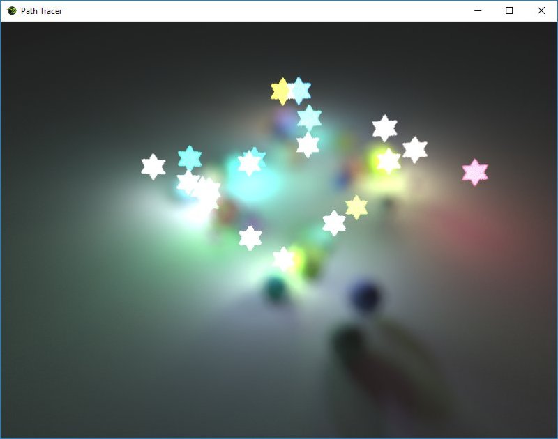
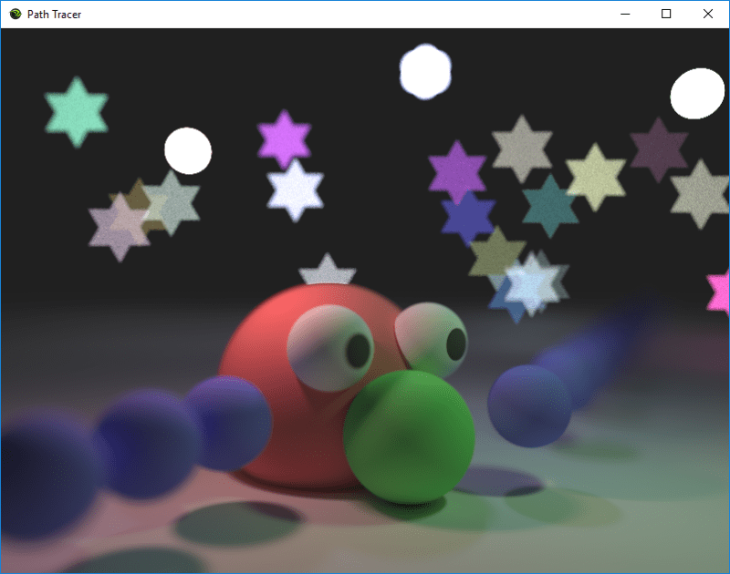
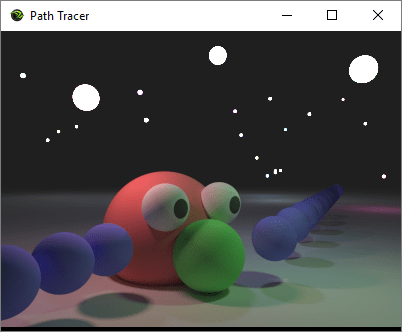
Let’s say you have a path tracer that can generate an image like this:
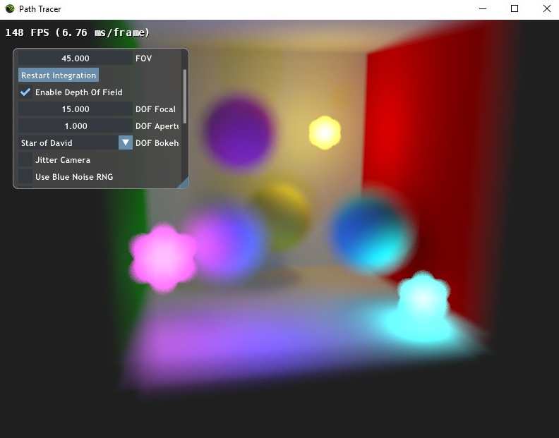
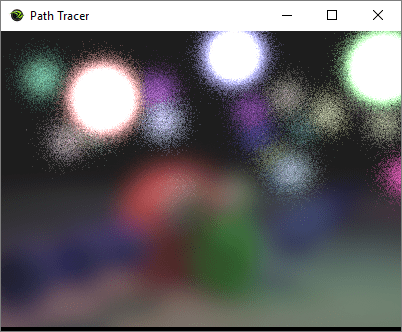
Adding depth of field (and bokeh) can make an image that looks like this:
The first image is rendered using an impossibly perfect pinhole camera (which is what we usually do in roughly real time graphics, in both rasterization and ray based rendering), and the second image is rendered using a simulated lens camera. This post is meant to explain everything you need to know to go from image 1 to image 2.
There is also a link to the code at the bottom of the post.
We are going to start off by looking at pinhole cameras – which can in fact have Bokeh too! – and then look at lens cameras.
If you don’t yet know path tracing basics enough to generate something like the first image, here are some great introductions:
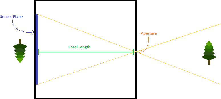
A pinhole camera is a box with a small hole – called an aperture – that lets light in. The light goes through the hole and hits a place on the back of the box called the “sensor plane” where you would have film or digital light sensors.
The idea is that the aperture is so small that each sensor has light hitting it from only one direction. When this is true, you have a perfectly sharp image of what’s in front of the camera. The image is flipped horizontally and vertically and is also significantly dimmer, but it’s perfectly sharp and in focus.
As you might imagine, a perfect pinhole camera as described can’t actually exist. The size of the hole is larger than a single photon, the thickness of the material is greater than infinitesimally small, and there are also diffraction effects that bend light as it goes through.
These real world imperfections make it so an individual sensor will get light from more than one direction through the aperture, making it blurrier and out of focus.
As far as aperture size goes, the smaller the aperture, the sharper the image. The larger the aperture, the blurrier the image. However, smaller apertures also let in less light so are dimmer.
This is why if you’ve ever seen a pinhole camera exhibit at a museum, they are always in very dark rooms. That lets a smaller aperture hole be used, giving a sharper and more impressive result.
When using a pinhole camera with film, if you wanted a sharp image that was also bright, you could make this happen by exposing the film to light for a longer period of time. This longer exposure time lets more light hit the film, resulting in a brighter image. You can also decrease the exposure time to make a less bright image.
Real film has non linear reaction to different wavelengths of light, but in the context of rendered images, we can just multiply the resulting colors by a value as a post effect process (so, you can adjust it without needing to re-render the image with different exposure values!). A multiplier between 0 and 1 makes the image darker, while a multiplier greater than 1 makes the image brighter.
It’s important to note that with a real camera, longer exposure times will also result in more motion blur. To counter act this effect, you can get film that reacts more quickly or more slowly to light. This lets you have the aperture size you want for desired sharpness level, while having the exposure time you want for desired motion blur, while still having the desired brightness, due to the films ISO (film speed).
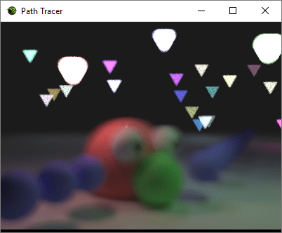
While aperture size matters, so does shape. When things are out of focus, they end up taking the shape of the aperture. Usually the aperture is shaped like something simple, such as a circle or a hexagon, but you can exploit this property to make for some really exotic bokeh effects. The image at the top of this post used a star of David shaped aperture for instance and this image below uses a heart shape.
Ultimately what is happening is convolution between the aperture and the light coming in. When something is in focus, the area of convolution is very small (and not noticeable). As it gets out of focus, it gets larger.
The last property I wanted to talk about is focal length. Adjusting focal length is just moving the sensor plane to be closer or farther away from the aperture. Adjusting the focal length gives counter intuitive results. The smaller the focal length (the closer the sensor plane is to the aperture), the smaller the objects appear. Conversely, the larger the focal length (the farther the sensor plane is from the aperture), the larger the objects appear.
The reason for this is because as the sensor plane gets closer, the field of view increases (the sensor can see a wider angle of stuff), and as it gets farther, the field of view decreases. It makes sense if you think about it a bit!
Pinhole Camera Settings Visualized
In the below, focal length and aperture radius are in “World Units”. For reference, the red sphere is 3 world units in radius. The path traced image is multiplied by an exposure multiplier before being shown on the screen and is only a post effect, meaning you can change the exposure without having to re-render the scene, since it’s just a color multiplier.
Here is a video showing how changing focal length affects the image. It ranges from 0.5 to 5.0. Wayne’s world, party time, excellent!
These next three images show how changing the aperture size affects brightness. This first image has an aperture size of 0.01 and an exposure of 3000.
This second image has an aperture size of 0.001 and the same exposure amount, making it a lot sharper, but also much darker.
This third image also has an aperture size of 0.001, but an exposure of 300,000. That makes it have the same brightness as the first image, but the same sharpness as the second image.
If you are wondering how to calculate how much exposure you need to get the same brightness with one aperture radius as another, it’s not too difficult. The amount of light coming through the aperture (aka the brightness) is multiplied by the area of the aperture.
When using a circular aperture, we can remember that the area of a circle is .
So, let’s say you were changing from a radius 10 aperture to a radius 5 aperture. The radius 10 circle has area of , and the radius 5 circle has an area of . That means that the radius 5 circle has 1/4 the area that the radius 10 circle does, which means you need to multiply your exposure by 4 to get the same brightness.
In the case of moving from radius 0.01 to 0.001, we are making the brightness be 1/100 of what it was, so we multiply the 3,000 by 100 to get the exposure value of 300,000.
Here is a video showing how aperture radius affects the sharpness of the image. The exposure is automatically adjusted to preserve brightness. Aperture radius ranges from 0.001 to 0.2.
In the next section we’ll talk about how to make different aperture shapes actually function, but as far as brightness and exposure goes, it’s the same story. You just need to be able to calculate the area of whatever shape (at whatever size it is) that you are using for your aperture shape. With that info you can calculate how to adjust the exposure when adjusting the aperture size.
Here are some different aperture shapes with roughly the same brightness (I eyeballed it instead of doing the exact math)
Circle:
Gaussian distributed circle:
Star of David:
Triangle:
Square:
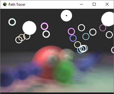
Ring:
Even though it’s possible to do bokeh with a pinhole camera as you can see, there is something not so desirable. We get the nice out of focus shapes, but we don’t get any in focus part of the image to contrast it. The reason for this is that pinhole cameras have constant focus over distance. Pinhole camera image sharpness is not affected by an object being closer or farther away.
To get different focus amounts over different distances, we need to use a lens! Before we talk about lenses though, lets talk about how you’d actually program a pinhole camera as we’ve described it.
Programming A Pinhole Camera With Bokeh
With the concepts explained let’s talk about how we’d actually program this.
First you calculate a ray as you normally would for path tracing, where the origin is the camera position, and the direction is the direction of the ray into the world. Adding subpixel jittering for anti aliasing (to integrate over the whole pixel) is fine.
At this point, you have a pinhole camera that has a infinitesimally small aperture. To make a more realistic pinhole camera, we’ll need to calculate a new ray which starts on the sensor plane, and heads towards a random point on the aperture.
Important note: the position of the aperture is the same as the camera position. They are the same point!
Calculating the Point on the Sensor Plane
We first find where the ray would hit the sensor plane if it were 1 unit behind the aperture (which will be a negative amount of time). We put that point into camera space, multiply the z of the camera space by the focal length (this moves the sensor plane), and then put it back into world space to get the actual world space origin of the ray, starting at the sensor plane.
To calculate the plane equation for the sensor plane, the normal for that plane is the camera’s forward direction, and a point on that plane is the camera position minus the camera’s forward direction. Calculating the equation for that plane is just:
From there, you do this to adjust the focal length and to get the world space starting position of the ray:
// convert the sensorPos from world space to camera space
float3 cameraSpaceSensorPos = mul(float4(sensorPos, 1.0f), viewMtx).xyz;

// elongate z by the focal length
cameraSpaceSensorPos.z *= DOFFocalLength;

// convert back into world space
sensorPos = mul(float4(cameraSpaceSensorPos, 1.0f), invViewMtx).xyz;
Now we know where the ray starts, but we need to know what direction it’s heading in still.
Calculating the Random Point on the Aperture
Now that we have the point on the sensor, we need to find a random point on the aperture to shoot the ray at.
To do that, we first calculate a uniform random point in a circle with radius “ApertureRadius”, since the aperture is a circle. Here is some code that does that (RandomFloat01() returns a random floating point number between 0 and 1):
If you wanted different shaped apertures for different shaped bokeh, you are only limited to whatever shapes you can generate uniformly random points on.
If we add that random offset to the camera position in camera space (multiply offset.x by the camera’s x axis, and offset.y by the camera’s y axis and add those to the camera position), that gives us a random point on the aperture. This is where we want to shoot the ray towards.
You can now use this ray to have a more realistic pinhole camera!
Brightness
If you want to be more physically correct, you would also multiply the result of your raytrace into the scene by the area of the aperture. This is the correct way to do monte carlo integration over the aperture (more info on monte carlo basics: https://blog.demofox.org/2018/06/12/monte-carlo-integration-explanation-in-1d/), but the intuitive explanation here is that a bigger hole lets in more light.
After you do that, you may find that you want to be able to adjust the aperture without affecting brightness, so then you’d go through the math I talk about before, and you’d auto calculate exposure based on aperture size.
When looking at the bigger picture of that setup, you’d be multiplying a number to account for aperture size, then you’d basically be dividing by that number to make it have the desired brightness – with a little extra to make it a little bit darker or brighter as the baseline brightness.
A more efficient way to do this would be to just not multiply by the aperture area, and apply an exposure to that result. That way, instead of doing something like dividing by 300,000 and then multiplying by 450,000, you would just multiply by 1.5, and it’d be easier for a human to work with.
Lens Cameras
Finally, onto lenses!
The simplest lens camera that you can make (and what I used) is to just put a convex lens inside the aperture.
A motivation for using lenses is that unlike pinhole cameras, you can increase the aperture size to let more light in, but still get a focused shot.
This comes at a cost though: there is a specific range of depth that is in focus. Other things that are too close or too far will appear blurry. Also, the larger the aperture, the smaller the “in focus range” will be.
From that perspective, it feels a bit silly simulating lenses in computer graphics, because there is no technical reason to simulate a lens. In computer graphics, it’s easier to make a sharper image than a blurry one, and if we want to adjust the image brightness, we just multiply the pixels by a constant.
Simulating a lens for depth of field and bokeh is purely a stylistic choice, and has nothing to do with a rendering being more correct!
How Convex Lenses Work
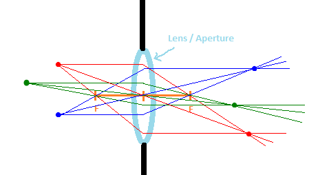
Convex lenses are also called converging lenses because they bend incoming light inwards to cross paths. Below is a diagram showing how the light travels from objects on the left side, through the lens, to the right side. The light meets on the other side of the lens at a focus point for each object. The orange “F” labels shows the focal distance of the lens.
If two points are the same distance from the lens on the axis perpendicular to the lens, their focal points will also be the same distance from the lens on that axis, on the other side of the lens.
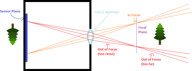
This means that if we had a camera with a sensor plane looking through a lens, that there would be a focal PLANE on the other side of the lens, made up of the focus points of each point for each sensor on the sensor plane. Things closer than the focus plane would be blurry, and things farther than the focus plane would be blurry, but things near the focus plane would be sharper.
The distance from the camera (aperture) to the focal plane is based on the focal distance of the lens, and also how far back the sensor plane is. Once you have those two values, you could calculate where the focal plane is.
There is a simpler way though for us. We can skip the middle man and just define the distance from the camera to the focal plane, pretending like we calculated it from the other values.
This is also a more intuitive setting because it literally tells you where an object has to be to be in focus. It has to be that many units from the camera to be perfectly in focus.
Going this route doesn’t make our renderer any less accurate, it just makes it easier to work with.
Nathan Reed (@Reedbeta) has this information to add, to clarify how focus works on lens cameras (Thanks!):
The thing you change when you adjust focus on your camera is the “image distance”, how far the aperture is from the film, which should be greater than or equal to the lens focal length.
The farther the aperture from the sensor, the nearer the focal plane, and vice versa. 1/i + 1/o = 1/f.
And this good info too:
“focal length” of a lens is the distance from film plane at which infinite depth is in sharp focus, and is a property of the lens, eg “18mm lens”, “55mm lens” etc. The focal length to sensor size ratio controls the FOV: longer lens = narrower FOV
Programming A Lens Camera With Bokeh
Programming a lens camera is pretty simple:
Calculate a ray like you normally would for a path tracer: the origin is the camera position, and the direction is pointed out into the world. Subpixel jitter is again just fine to mix with this.
Find where this ray hits the focal plane. This is the focal point for this ray
Pick a uniform random spot on the aperture
Shoot the ray from the random aperture position to the focal point.
That’s all there is to it!
You could go through a more complex simulation where you shoot a ray from the sensor position to a random spot on the aperture, calculate the refraction ray, and shoot that ray into the world, but you’d come up with the same result.
Doing it the way I described makes it no less accurate(*)(**), but is simpler and computationally less expensive.
* You’ll notice that changing the distance to the focal plane doesn’t affect FOV like changing the focal distance did for the pinhole camera. If you did the “full simulation” it would.
** Ok technically this is a “thin lens approximation”, so isn’t quite as accurate but it is pretty close for most uses. A more realistic lens would also have chromatic aberration and other things so ::shrug::
You can optionally multiply the result of the ray trace by the aperture size like we mentioned in the pinhole camera to make the brightness be properly affected by aperture size. If you’d rather not fight with exposure multiplier calculations as you change aperture size though, feel free to leave it out.
This video shows the effect of the aperture size changing. Notice that the area in focus is smaller with a larger aperture radius.
This video shows the effect of the focal distance changing. Nothing too surprising here, it just changes what depth is in focus.
Photography is a Skill
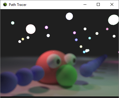
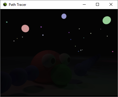
Even after I had things implemented correctly, I was having trouble understanding how to set the parameters to get good Bokeh shots, as you can see from my early images below:
Luckily, @romainguy clued me in: “Longer focals, wider apertures, larger distance separation between subjects”
So what I was missing is that the bokeh is the stuff in the background, which you make out of focus, and you put the focal plane at the foreground objects you want in focus.
It’s a bit strange when you’ve implemented something and then need to go ask folks skilled in another skill set how to use what you’ve made hehe.
Other Links
Here’s some other links I found useful while implementing the code and writing this post:
The path tracer uses nvidia’s “Falcor” api abstraction layer. As best as I can tell, just pulling down falcor to your machine and compiling it registers it *somewhere* such that projects that depend on falcor can find it. I’m not really sure how that works, but that worked for me on a couple machines I tried it on strangely.
I wish I had a more fool proof way to share the code – like if it were to download the right version of falcor when you try to build it. AFAIK there isn’t a better way, but if there is I would love to hear about it.


 .
. , and the radius 5 circle has an area of
  . That means that the radius 5 circle has 1/4 the area that the radius 10 circle does, which means you need to multiply your exposure by 4 to get the same brightness.


 .
.