Inverting the CDF lets you convert from uniform to non uniform distributions, but you can also use the CDF to convert from the non uniform distribution to a uniform distribution.
This means that just like you can square root a uniform random number between 0 and 1 to get a “linear” distributed random number where larger numbers are more likely, you could also take linear distributed random numbers and square them to get uniform random numbers.
float UniformToLinear(float x)
{
	// PDF In:  y = 1
	// PDF Out: y = 2x
	// ICDF:    y = sqrt(x)
	return std::sqrt(x);
}

float LinearToUniform(float x)
{
	// PDF In:  y = 2x
	// PDF Out: y = 1
	// ICDF:    y = x*x
	return x*x;
}
This can be useful when you use a two tap FIR filter which gives a triangle distribution out. You can adapt the LinearToUniform function to convert the first half of a triangle distribution back to uniform, the values between 0 and 0.5. For the second half of the triangle distribution, you can subtract it from 1.0, to get values between 0 and 0.5 again, convert from linear to uniform, and then subtract it from 1.0 again to flip it back around.
float TriangleToUniform(float x)
{
	if (x < 0.5f)
	{
		x = LinearToUniform(x * 2.0f) / 2.0f;
	}
	else
	{
		x = 1.0f - x;
		x = LinearToUniform(x * 2.0f) / 2.0f;
		x = 1.0f - x;
	}
	return x;
}
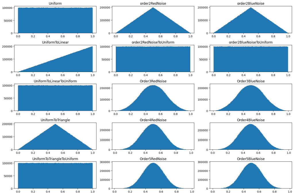
Let’s see how this works out in practice. In the first column below, it shows uniform being converted to linear and triangle, and back, to show that the round trip works.
In the second column, it shows red noise (low frequency random numbers) being made by adding two random numbers together, and then being made into uniform noise by converting from triangle to unfirom. It then also shows higher order red noise histograms.
The third column shows the same, but with blue noise (high frequency random numbers.
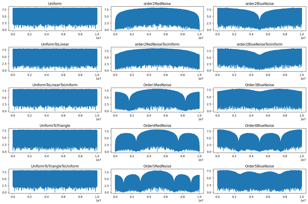
Here are the DFTs of the above, showing that the frequency content stays pretty similar through these various transformations.
So while we have the ability to convert 2 tap filtered noise from triangular distributed noise to uniform distributed noise, what about higher tap counts that give higher order binomial distributions?
It turns out the binomial quantile function (inverse CDF) doesn’t have a closed form that you can evaluate symbolically, which is unfortunate. Maybe two taps is good enough.
Here are 20 values of each noise type to let you see what kind of values they actually have. The numbers are mapped to be between 0 and 1 even though these noise types naturally have other ranges. Order 2 red noise goes between 0 and 2 for example, and order 2 blue noise goes between -1 and 1.
This post is the result of a collaboration between myself and R4 Unit on mastodon (https://mastodon.gamedev.place/@R4_Unit@sigmoid.social/109810895052157457). R4 Unit is actually the one who showed me you could animate blue noise textures by adding the golden ratio to each pixel value every frame too some years back 🙂
Fibonacci and the golden ratio are often used interchangeably, which can be confusing but this is due to them being two sides of the same coin. If you divide a Fibonacci number by the previous Fibonacci number, you will get approximately the golden ratio 1.6180339887.
The first few Fibonacci numbers are
1, 1, 2, 3, 5, 8, 13, 21, 34, and 55
Starting at the second 1 and dividing each number by the last number gives
1, 2, 1.5, 1.666, 1.6, 1.625, 1.615, 1.619, and 1.6176
This converges to the golden ratio and is exactly the golden ratio at infinity.
The golden ratio appears as the greek letter “phi,” which rhymes with pi and pie. It looks like φ (lowercase) or ϕ (uppercase).
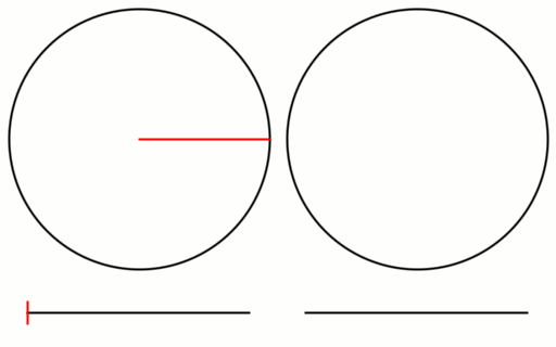
You’ll see circles talked about a lot in this post and might wonder why. In 1D sampling, we sample a function for x between 0 and 1. Our actual function might want us to sample a different domain (like say between 1 and 4), but for simplicity’s sake, we generate points between 0 and 1 and map them to the different values if needed. When generating low discrepancy sequences, we want to generate values between 0 and 1 through “some process.” When values outside 0 to 1 are generated, modulus brings them back in. It’s as if we rolled our 0 to 1 number line segment into a circle where 1 and 0 connect. A value of 1.5 goes around the circle 1.5 times and lands at the 0.5 mark. Our line segment is basically a circle.
You may wonder about the difference between a low discrepancy sequence and a low discrepancy set. A low discrepancy sequence is a sequence of points with an ordering, and Wikipedia states that any subsequence starting at the first index is also low discrepancy (https://en.wikipedia.org/wiki/Low-discrepancy_sequence). A low discrepancy set is a set of points where all points must be used before they are low discrepancy.
If you are wondering what low discrepancy means, discrepancy is a measurement of how evenly spaced the points are. Low discrepancy sequences have nearly evenly spaced points, but not quite. This is a valuable property for sampling, with one reason being that perfectly evenly spaced points are subject to aliasing. At the same time, completely random (uniform white noise) will form clumps and voids, have a high discrepancy, and leave parts of the sampling domain unsampled.
We’ll be talking about the golden ratio low discrepancy sequence next, which has an ordering and is low discrepancy at each step.
The Golden Ratio Low Discrepancy Sequence
The golden ratio low discrepancy sequence (LDS) is a 1D sampling sequence with some excellent properties. When viewing on a number line, or a circle, the following sample always appears in the largest gap. This is true no matter what index you start in the sequence, which is a bit of a mind-bender. See the animation below.
Generating the golden ratio sequence is simple and computationally inexpensive:
Multiplying the index by the golden ratio will cause floating point inaccuracies that affect the sequence as the index gets larger, so it’s better to have a function that gives you the next value in the sequence, that you can call repeatedly.
We can realize we only care about the fractional part of the golden ratio and subtract one from it. This value is called the golden ratio conjugate and is the value of 1/φ, and it is every bit as irrational as the golden ratio.
For best results, you can supply a random floating point number between 0 and 1 as the first value in the sequence.
The golden ratio LDS has excellent convergence for 1D integration (* asterisk to be explained in next section), but the samples aren’t in a sorted order. Looking at the number line, you can see that the samples come in a somewhat random (progressive) order. If these sampling positions correspond to different places in memory, this is not great for memory caches.
Furthermore, some sampling algorithms require you to visit the sample points in a sorted order – for instance, when ray marching participating media and alpha compositing the samples to make the final result. Maybe it would be nice if they were in a sorted order?
Wanting a sorted version of the golden ratio LDS, I tried to solve it myself at first. I analyzed the gaps between the numbers for different sample counts and found some interesting identities involving different powers of φ, 1/φ, and 1-1/φ. I found a pattern and was able to describe this as a binary sequence, with rules for how to split the binary sequence to get the next sample. Then I got stuck, unsure how to use this knowledge to make sample points in order.
I shared some tidbits, and R4 Unit asked what I was up to. After explaining, getting some great info back, having further conversations, and implementing in parallel, the solution came into focus.
If you place marks on a circle at multiples of some number of degrees, there will ever be at most three distinct distances between points on the circle (https://en.wikipedia.org/wiki/Three-gap_theorem)
If using the golden angle, and a Fibonacci number of points, there are only ever two distances between points, and you can calculate them easily. Furthermore, if starting at a point on the circle, the “Infinite Fibonacci Word” will tell you the step size (0 = big, 1 = small) to take to get to the next point in the circle for the “Golden Angle Low Discrepancy Sequence.” See the bullet point here about unit circles and the golden angle sequence https://en.wikipedia.org/wiki/Fibonacci_word#Other_properties. We divide the sequence by 2pi to get 0 to 1 on a number line instead of 0 to 2pi as radians on a circle. The golden angle low discrepancy sequence is generated the same way as the golden ratio low discrepancy sequence but uses 0.38196601125 as the constant (2-φ, or 1/φ^2).
You can start at any point of the circle. It just rotates the circle. That means that when we generate our sequence, we can start at any random point 0 to 1 as a randomizing offset, and the quality of the sequence is unaltered.
static const float c_goldenRatio = 1.61803398875f;
static const float c_goldenRatioConjugate = 0.61803398875f; // 1/goldenRatio or goldenRatio-1

float FibonacciWordSequenceNext(float last, float big, float small, float& run)
{
    run += c_goldenRatio;
    float shift = std::floor(run);
    run -= shift;
    return last + ((shift == 1.0f) ? small : big);
}

// big can be set to 1.0f / float(numSamples), but will return >= numSamples points if so.
std::vector<float> Sequence_FibonacciWord(float big)
{
    std::vector<float> ret;
    float small = big * c_goldenRatioConjugate;
    float run = c_goldenRatioConjugate;
    float sample = 0.0f;
    while (sample < 1.0f)
    {
        ret.push_back(sample);
        sample = FibonacciWordSequenceNext(sample, big, small, run);
    }
    return ret;
}
Generating the next sample is amazingly simple. If you print out the value of “shift,” you’ll see that it is the Infinite Fibonacci Word, which decides whether to add the small or large gap size to get to the next point.
Other Implementation Details
In practice, there is a challenge with this sampling sequence. If you ask for N samples, it will usually return slightly more samples than that.
You might think it’d be ok to truncate them and just throw out the extra ones. If you do that, your convergence will be bad due to areas not being sampled at the end of your sampling domain.
You may decide you could throw out the extra ones and renormalize the point set to span the 0 to 1 interval by stretching it out, even being careful to preserve the ratio of the gap at the end between the last sample and 1.0. Unfortunately, if you do that, your convergence is still bad.
I tried both things, and the convergence degraded such that it was no longer competitive. It was a no-go.
In the sample code, I tell it to generate N samples. If it comes back with too many, I decrement N and try again. This repeats until the right number of samples is returned, or going any lower would make me not have enough samples.
If there are too many samples at this point, I truncate and divide all samples by the first sample thrown away. This rescales the sequence to fill the full 0 to 1 domain.
This process makes the results used in the next section and is what I found to be best.
This is a very costly operation, speculatively generating sequences of unknown length in a loop until we get the right amount, but this is something that could be done in advance. You can know that if you want a specific N number of samples, you say to generate M samples instead and divide each sample by a constant k which is the sample that comes right after the last one.
This might be a pain and require a couple more shader constants or magic numbers, but consider it the cost of better convergence. The things we do for beauty!
One last item… when you implement this, you need a way to apply an offset to the sequence, using a blue noise texture or whatever else you might want to use. I had good luck multiplying my 0 to 1 random value by the number of indices in my sequence, and using the fractional part of the index as a multiplier of the either big or small sized gap for that index. It felt like that might not work well, because each index is either a large or small gap, and this treats them as the same size, but it didn’t damage the quality in my testing, so that was nice.
Convergence
Now that we can make the sequence, let’s see if it is any good.
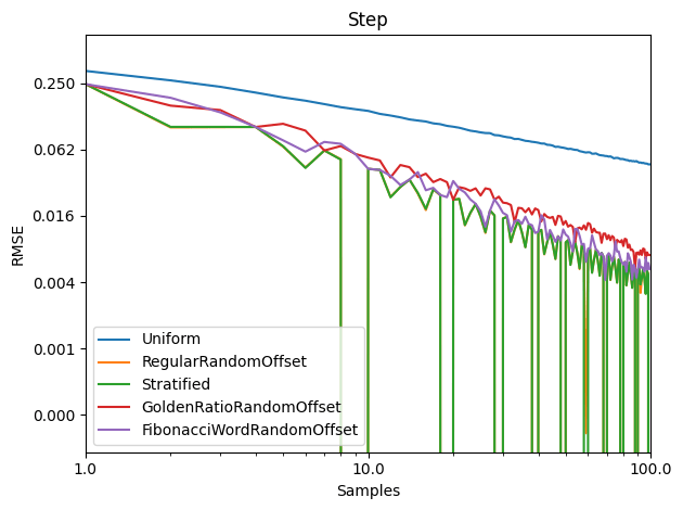
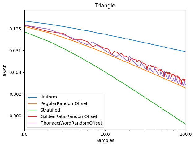
I tested the usual choices for 1D integration against three functions, did this 10,000 times, and graphed the RMSE.
Sampling Types:
Uniform – Uniform random white noise.
RegularRandomOffset – Regularly spaced sampling (index/N), with a single global random offset added to all the samples to shift the sequence a random amount around the circle for each test.
Stratified – Regular spaced sampling, but with a random offset added to each sample ((index + rand01()) / N).
GoldenRatioRandomOffset – The golden ratio LDS, with a single global random offset added to all the samples to shift the sequence a random amount around the circle for each test.
FibonacciWordRandomOffset – The sequence described in this post, with a single global random offset added to all the samples to shift the sequence a random amount around the circle for each test.
I also tested VanDerCorput base two and base three. Their results were similar to the golden ratio results and are unsorted so only cluttered the graph, and are thus omitted.
Sine: y = sin(pi * x)
Step: y = (x < 0.3) ? 1.0 : 0.0
Triangle: y = x
Well bummer… it turns out not to be so great vs stratified sampling or regular spaced sampling with a random global shift.
The power in the 1d golden ratio sequence is that for any number of samples you have, it is pretty good sampling, and you can add more to it. This is useful if you don’t know how many samples you are going to take, or if you want to have a good (progressive) result as you take more samples.
If you know how many samples you want, it looks like it’s better to go with stratified, or regularly spaced samples with a random global shift.
When I was early in this journey I made a typo in my code where it only tested N-1 samples in these convergence graphs instead of the full N samples. In that situation, golden ratio worked well because it works fine for any number of samples from 0 to M. The sorted golden ratio ended up working as well because it is “well spaced” for a fibonacci number of samples, but otherwise, the samples bunch up a little bit at the end, so removing the last sample wasn’t very damaging. Due to this unfortunate typo, I saw from early on that a sorted golden ratio sequence would be real valuable (like for ray marching fog volumes), to get better convergence while still being able to get samples in order.
This one didn’t work out, but oh well, onto the next thing 😛