Quantum Computing For Programmers Part Ib: Bloch Sphere

If you read anything on quantum computing you are extremely likely to see the Bloch sphere, so it’s probably important to explain what it is and how it works.

Image from wikipedia: Wikipedia: Qubit

The Bloch sphere is a way of visually representing a qubit.

The north pole is the $|0\rangle$ state, and the south pole is the $|1\rangle$ state. The Z axis is vertical and runs from the $|0\rangle$ to the $|1\rangle$ state. A qubit’s state is represented by a point on the sphere.

If you read the last post, you might remember that there was a Pauli-Z gate which changed the phase of a qubit without changing it’s probability, as well as a more generalized version of the phase changing gate which also just rotated around the Z axis. Looking at the bloch sphere, you can see why that is true! Rotating a point around the Z axis moves it around the sphere horizontally, but it doesn’t make it any closer or farther to either the north or south pole. Since the distance to the poles is preserved, the probability of being one or the other stays the same, even though the phase changes.

The not gate, aka the Pauli-X gate, rotated a point around the X axis 180 degrees. Looking at the sphere, you could see how that would change a $|1\rangle$ to a $|0\rangle$ , or otherwise flip the probabilities & amplitudes of the states.

The Pauli-Y gate is a little more complex though (pun intended!) as it mapped $|0\rangle$ to $i|1\rangle$ and $|1\rangle$ to $-i|0\rangle$ by rotating 180 degrees around the Y axis. You may wonder how $|1\rangle$ and $i|1\rangle$ can both refer to the south pole, but the situation there is that every point EXCEPT the poles have a unique representation. So, they really do both refer to the south pole.

To find where a qubit sits on the sphere, the first step is to figure out the spherical coordinates theta ( $\theta$ ) and phi ( $\phi$ ) values, which you can then convert to a 3d point.

Start with whatever qubit you have in this form, where you know what the values for alpha ( $\alpha$ ) and beta ( $\beta$ ) are:
$|\psi\rangle = \alpha|0\rangle + \beta|1\rangle$

You can also write a qubit as:
$|\psi\rangle = \cos\left(\tfrac{\theta}{2}\right) |0 \rangle \, + \, e^{i \phi} \sin\left(\tfrac{\theta}{2}\right) |1 \rangle$

Or like this, with less euler, and more trig:
$|\psi\rangle = \cos\left(\tfrac{\theta}{2}\right) |0 \rangle \, + \, ( \cos \phi + i \sin \phi) \, \sin\left(\tfrac{\theta}{2}\right) |1 \rangle$

You can then set your known alpha and beta values to the trig (or euler) based equations:
$\alpha = \cos\left(\tfrac{\theta}{2}\right)$
$\beta = \, ( \cos \phi + i \sin \phi) \, \sin\left(\tfrac{\theta}{2}\right)$

and then solve for theta and phi (I wave my hands a bit here).

Once you have the theta and phi values figured out, you can convert that to a unit distance 3d point representing a point on the sphere by using the below, which describes the X,Y,Z components of the point:
$(\sin \theta \cos \phi, \; \sin \theta \sin \phi, \; \cos \theta)$

Hopefully this explanation makes enough sense that if you encounter the bloch sphere, or things talking about rotations on the bloch sphere, you won’t be too lost 😛

Ok… time to move on to multiple qubit quantum circuits so we can do more interesting things and perhaps analyze the most well known quantum algorithms!

Quantum Computing For Programmers Part I: One Qubit

Are you a programmer? Do you have interest in learning how quantum computing works? Does hard core math and crazy abstract “philosophical” type physics questions about the nature of reality make you feel like you could never understand quantum computing?

If so, me too, welcome to the club! We are programmers, not mathematicians or physicists, but we are masters of our realm – computation and logic. With that, I say that quantum computing is ultimately meant for us, since it is computing and programming, so lets figure it out and do some interesting stuff 😛

Before we start, I want to mention that these posts should be able to be read stand alone, but if you want to get into the deeper details, you probably want to give this list of references I’m using a read at some point. Perhaps before reading my posts, or after, or both!
Quantum Computing References

Lastly, to be clear, quantum computers seem like they are a long way off from being common place objects. These posts will show how quantum computers work, and allow you to simulate quantum computers on your own computer with some simple C++. The code won’t run as fast as it would on a real quantum computer (obviously!), but it should let you better understand how Quantum Computing (QC) works and let you explore and experiment on your own machine.

Probabilities (aka SuperPositons)

At the core of QC is the qubit. A qubit is like a regular bit, in that it can have the value of 0 or 1, but unlike a regular bit, it can also be somewhere in the middle where it has a probability of being in each state.

That might sound strange, but think of a qubit like a coin. It can be heads up, or it can be heads down, or it can be in the air, waiting to land heads up or heads down.

When the coin is in the air, if it is perfectly balanced, it has a 50/50 chance of becoming heads or tails.

If the coin is not perfectly balanced (no real coin can be perfectly balanced!), it will have some bias towards heads or towards tails so will not be a pure 50/50 chance of heads or tails.

While the coin is on the ground, it is either a heads (0) or a tails (1), but while it’s in the air, you can imagine that it is a superposition of 0 and 1. When it lands, that superposition will collapse into a 0 or 1 value, which is also what happens when you “observe” or measure a qubit.

One interesting thing about quantum computing, and where part of it’s power comes from is that you can perform logic on superpositional values in a way that when you have your final superpositional result, you can measure it and get the result from your logic circuit as if the values had been fixed all the way through the system, instead of being in superpositions.

The bummer about this though is that since it’s all based on probabilities, your answer has a chance of being not the value you wanted to get. Quantum circuits / quantum algorithms will try to combat this by doing operations iteratively to make the probability of the desired answer go up, and the probability of the undesired answers go down.

They can also run the quantum algorithm multiple times, to take multiple samples and be more sure about their results.

You still with me? Pretty simple so far right?

Before moving on I also wanted to mention that regular computers – like the one you are using right now – also have a greater than zero chance that they will give you the wrong answer to a calculation. The error rate can increase when the components are too hot, but even otherwise, a stray particle of background radiation could hit your cpu and flip a bit, giving you the wrong answer. You could fight this by doing every calculation 3 times and going with majority rules, but even then, if two bits get flipped, the majority will be wrong. Nothing you can do can completely eliminate the random chance that your calculations will come up with the wrong answer, but the chances are low enough that we rely on computers to do the right things, even in the most critical of situations (like, not starting a thermonuclear war).

With quantum computers you could get that same level of assurance. You can never completely eliminate the chance that a calculation is wrong, but you can definitely be sure with as much accuracy as you can with a standard computer, so that shouldn’t really be an issue in practice, for the cases where you need “certainty”.

Probability Vectors (aka Amplitude Vectors)

Using the coin flip scenario above, we could describe the probability of a coin landing heads or tails as a vector where the first element is the chance that it will land heads, and the second element is the chance that it will land tails.

A perfectly balanced coin would look like this for instance: $[0.5,0.5]$

If the coin was 75% likely to land heads, and only 25% likely to land tails the vector would look like this: $[0.75,0.25]$

You might notice that the elements of the vector have to add up to 1. This makes sense because there are only two options and one of the two MUST happen (unless it lands perfectly on edge), so they better add up to 1! The technical term for this is that the vector must have an L1 Norm of 1.

Qubits describe their probabilities a little bit differently though. Instead of storing the probability of them being 0 or 1, they store what’s called the amplitude, which when squared gives the probability. Doing this lets them do something really important that I’ll talk about lower down, but for now, you can hopefully just accept that this is how it works.

Consider a qubit having a 50% chance that it’s a 0, and a 50% chance that it’s a 1. We need some number that when squared gives 0.5 aka 1/2. That value is $1/\sqrt{2}$ .

So, for a qubit that has an even chance of being a 0 or 1, a vector to represent it is $[1/\sqrt{2}, 1/\sqrt{2}]$ .

Then, a vector describing a qubit that has a 75% chance being a 0 and a 25% chance of being a 1 would be $[\sqrt{3}/2, 1/2]$ . If you square the first number you can see that you get 3/4 (75% chance) and squaring the second number gives you 1/4 (25% chance).

I got those vectors by solving the simple equation:
$x^2 = P$

Where $P$ is the desired probability from 0 to 1.

You might now notice that the length of a qubit amplitude vector has to be 1. In other words, it’s a normalized vector. The technical term for this is that the vector must have an L2 norm of 1.

Still nothing too crazy going on…

Ket Notation

There is some notation you’ll come across a lot when reading about quantum computing / mechanics / etc that looks like this:
$1/\sqrt{2}(|0\rangle + |1\rangle)$

That is “Ket Notation” and comes from “Bra-Ket Notation”. It’s bark is worse than it’s bite.

If you multiply it out, you get this:
$1/\sqrt{2} * |0\rangle + 1/\sqrt{2} * |1\rangle$

All that means is that the “0” state of the vector has an amplitude of $1/\sqrt{2}$ and so does the “1” state. Writing that as a vector, we get what we already saw above for the qubit which had 50/50 odds of being a 0 or a 1:
$[1/\sqrt{2}, 1/\sqrt{2}]$

Here is the ket notation for the qubit which had a 75% chance of being a 0 and a 25% chance of being a 1:
$1/2(\sqrt{3}|0\rangle + |1\rangle)$

You can multiply that out to get this:
$\sqrt{3}/2*|0\rangle + 1/2*|1\rangle$

Which translates to the vector we saw before:
$[\sqrt{3}/2, 1/2]$

Lastly, you might see it shown like this:
$|0\rangle$

All that means is that the “0” state is 1. Since the “1” state isn’t listed, it has a value of 0. That is the same as this vector:
$[1, 0]$

Ket notation is used because you only have to list the states that actually have values, and not the ones that have zeros, making a more compact representation. That will be more useful when we move into a larger number of qubits.

Note that the mapping of which state belongs to which spot in the vector is completely arbitrary. I chose to make the left value be the “0” state and the right value be the “1” state, but it really doesn’t matter how you define it, so long as you are consistent.

Phase

Phase is the reason that qubits store amplitude, which square to probabilities, instead of storing probabilities themselves.

I said that the amplitude vector for a qubit which has a 50/50 chance of being a 0 or a 1 was this:
$[1/\sqrt{2}, 1/\sqrt{2}]$

I lied a bit though, and that is only one possible answer. Here’s another that has a 50/50 chance:
$[-1/\sqrt{2}, 1/\sqrt{2}]$

This gets interesting when you add two vectors together. First lets add two amplitude vectors which have the same phases for each state:
$[1/\sqrt{2}, 1/\sqrt{2}] + [1/\sqrt{2}, 1/\sqrt{2}] = [\sqrt{2}, \sqrt{2}]$

Each component added together.

Now, let’s add two amplitude vectors where the $|1\rangle$ state has opposite phase in one of the vectors:
$[1/\sqrt{2}, 1/\sqrt{2}] + [1/\sqrt{2}, -1/\sqrt{2}] = [\sqrt{2}, 0]$

You can see that the $|0\rangle$ states added together while the $|1\rangle$ states subtracted and resulted in zero.

This is called destructive interference, and is one of the things that makes quantum computing powerful. We can change a qubit’s phase without affecting it’s value (or probability of values).

I left out another important amplitude vector for describing a qubit that has a 50/50 chance of being a 0 or a 1:
$[1/\sqrt{2}, 1/\sqrt{-2}]$

Which can also be written as:
$[1/\sqrt{2}, 1/(\sqrt{2}*i)]$

Yep, that is an imaginary number in the 1 state!

Since amplitude squared is probability, it means we can also use imaginary numbers for amplitude vector values. If you know that the term phase relates to angles and rotations, you might want to have a look at these two things to follow the rabbit hole a bit deeper. Totally optional (;
Using Imaginary Numbers To Rotate 2D Vectors
Wikipedia: Bloch Sphere

However, since imaginary numbers can be involved, squaring amplitudes to get probabilities isn’t enough. Like for example with the vector $[0,i]$ , if you square the $|1\rangle$ state to get the probability, you get -1, or -100%. That isn’t right!

The real operation to getting probability from amplitude is you multiply the amplitude by it’s complex conjugate. In other words, if you have a complex number, you multiply the imaginary part by -1 to get the conjugate, and multiply by that.

As an example, if you have $3+5i$ , the complex conjugate is $3-5i$ .

In the example of the vector $[0,i]$ , you get the probability of the $|1\rangle$ state by multiplying $i$ by $-i$ to get 1, or 100%.

Complex conjugate sounds scary, but hopefully you can see it isn’t as scary as it sounds. You just flip the sign of the imaginary component of the complex number.

Common One Qubit Logic Gates

It’s finally time to dive into some logic gates so we can actually do some quantum programming!

Real quickly I want to mention that we are going to be simulating quantum computing by multiplying the qubit amplitude vectors by matrices. The matrices themselves are unitary matrices, which preserves the length of the vectors (keeping them normalized).

One requirement of quantum gates is that they must be reversible, and unitary matrices are also reversible.

The matrices are square matrices and their dimensions will always be 2^N by 2^N where N is the number of qubits involved in the quantum circuit. With a single qubit, that means we will be working with 2×2 matrices which is fairly small.

When working with more qubits the size of the matrix grows very quickly though. Quantum computing is very fast at doing these “matrix multiplies” and is part of where their power comes from. Large matrix multiplies will be slow for us on regular (classical) computers, but the quantum computers would be able to do them very quickly. That’s where the difference is in our simulations versus the real deal.

Anyways, let’s get onto some specific logic gates! (These are from Wikipedia: Quantum Gate)

Not Gate (Pauli-X Gate)

This is a not gate, but is also described as a 180 degree rotation around the x axis of the bloch sphere.

$\begin{bmatrix} 0 & 1 \\ 1 & 0 \\ \end{bmatrix}$

You might notice that it looks like a backwards identity matrix. That is exactly how it works too… if you multiply a 2 element vector by that matrix, it will flip the elements in that vector!

In the case of our qubit amplitude vectors, this has the result of swapping the probability that the qubit will be 0, with the probability that the qubit will be 1.

If the qubit is not in a superposition, and instead is actually just a 0 or a 1, it will act exactly like a traditional NOT gate and flip it from one value to the other.

If the qubit is in a superposition, it will just flip the probabilities of each state.

This maps the $|0\rangle$ state to $|1\rangle$ and vice versa.

Pauli-Y Gate

This is described as a 180 degree rotation around the y axis of the bloch sphere, and maps $|0\rangle$ to $i|1\rangle$ and $|1\rangle$ to $-i|0\rangle$ .

$\begin{bmatrix} 0 & -i \\ i & 0 \\ \end{bmatrix}$

It’s like a NOT but also adjusts phase.

Pauli-Z Gate

This is described as a 180 degree rotation around the z axis of the bloch sphere. All it does in practice is negate the phase of the $|1\rangle$ state.

$\begin{bmatrix} 1 & 0 \\ 0 & -1 \\ \end{bmatrix}$

General Phase Adjustment Gates

You can adjust the phase of individual gates by using a matrix like this one, which is a more general version of the Pauli-Z gate, and adjusts the phase of of the $|1\rangle$ state to whatever value is desired, without affecting the probabilities of the qubit values.

$\begin{bmatrix} 1 & 0 \\ 0 & e^{i\theta} \\ \end{bmatrix}$

The value $e^{i\theta}$ ends up being a complex number, that can also be written like this:
$cos(\theta)+i sin(\theta)$

where $\theta$ is any angle in radians.

You’ll find that circuits commonly only adjust the $|1\rangle$ state. This is because the absolute phase of the individual states don’t matter (since they don’t affect probabilities), but what does matter is the difference in phase between the $|0\rangle$ state and the $|1\rangle$ state, since that can cause constructive or destructive interference. For this reason, you’ll often see the $|0\rangle$ state without a phase value, and only the $|1\rangle$ state will get it’s phase modified during calculations.

Hadamard Gate (Interesting Gate!)

Ok so the NOT gate is somewhat useful. You are probably thinking the others might come in handy if you need to adjust the phase of a qubit, but so far, nothing has been that spectacular for single qubit gates.

Well, here’s the more interesting gate.

What this gate does is if you pass it a pure 0 or 1, it will output a value that has a 50% chance of being a 0 or a 1.

The interesting part happens when you put that output through a Hadamard gate again – you get the original value of 0 or 1 out!

It can do this because it stores the info about the original value as phase information. When the input value is $|0\rangle$ , the Hadamard gate outputs $[1/\sqrt{2}, 1/\sqrt{2}]$ which has matching phases for each state. When the input value is $|1\rangle$ , the gate outputs $[1/\sqrt{2}, -1/\sqrt{2}]$ which has opposite phases for each state.

$1/\sqrt{2} \begin{bmatrix} 1 & 1 \\ 1 & -1 \\ \end{bmatrix}$

This gate is a crucial part in both Grover’s algorithm – which can search an unsorted list in $O(\sqrt{N})$ , as well as in Shor’s algorithm, which can factor large numbers much faster than classical computers, putting certain types of cryptography at risk for being cracked by quantum computers.

It has some other uses too, which you can check out here:
Does a Hadamard Gate have uses outside of pure and evenly mixed states?

Code

Here is some example code to show some single qubit circuits in action.

#include <stdio.h>
#include <array>
#include <complex>

typedef std::array<std::complex<float>, 2> TQubit;
typedef std::array<std::complex<float>, 4> TComplexMatrix;
const float c_pi = 3.14159265359f;

//=================================================================================
static const TQubit c_qubit0 = { 1.0f, 0.0f };  // false aka |0>
static const TQubit c_qubit1 = { 0.0f, 1.0f };  // true aka |1>
static const TQubit c_qubit01_0deg = { 1.0f / std::sqrt(2.0f), 1.0f / std::sqrt(2.0f) }; // 50% true. 0 degree phase
static const TQubit c_qubit01_180deg = { 1.0f / std::sqrt(2.0f), -1.0f / std::sqrt(2.0f) }; // 50% true. 180 degree phase

// A not gate AKA Pauli-X gate
// Flips false and true probabilities (amplitudes)
// Maps |0> to |1>, and |1> to |0>
// Rotates PI radians around the x axis of the Bloch Sphere
static const TComplexMatrix c_notGate =
{
    {
        0.0f, 1.0f,
        1.0f, 0.0f
    }
};
static const TComplexMatrix c_pauliXGate = c_notGate;

// Pauli-Y gate
// Maps |0> to i|1>, and |1> to -i|0>
// Rotates PI radians around the y axis of the Bloch Sphere
static const TComplexMatrix c_pauliYGate =
{
    {
        { 0.0f, 0.0f }, { 0.0f, -1.0f },
        { 0.0f, 1.0f }, { 0.0f, 0.0f }
    }
};

// Pauli-Z gate
// Negates the phase of the |1> state
// Rotates PI radians around the z axis of the Bloch Sphere
static const TComplexMatrix c_pauliZGate =
{
    {
        1.0f, 0.0f,
        0.0f, -1.0f
    }
};

// Hadamard gate
// Takes a pure |0> or |1> state and makes a 50/50 superposition between |0> and |1>.
// Put a 50/50 superposition through and get the pure |0> or |1> back.
// Encodes the origional value in the phase information as either matching or
// mismatching phase.
static const TComplexMatrix c_hadamardGate =
{
    {
        1.0f / std::sqrt(2.0f), 1.0f / std::sqrt(2.0f),
        1.0f / std::sqrt(2.0f), 1.0f / -std::sqrt(2.0f)
    }
};

//=================================================================================
void WaitForEnter ()
{
    printf("nPress Enter to quit");
    fflush(stdin);
    getchar();
}

//=================================================================================
TQubit ApplyGate (const TQubit& qubit, const TComplexMatrix& gate)
{
    // multiply qubit amplitude vector by unitary gate matrix
    return 
    {
        qubit[0] * gate[0] + qubit[1] * gate[1],
        qubit[0] * gate[2] + qubit[1] * gate[3]
    };
}

//=================================================================================
int ProbabilityOfBeingTrue (const TQubit& qubit)
{
    float prob = std::round((qubit[1] * std::conj(qubit[1])).real() * 100.0f);
    return int(prob);
}

//=================================================================================
TComplexMatrix MakePhaseAdjustmentGate (float radians)
{
    // This makes a gate like this:
    //
    // [ 1  0             ]
    // [ 0  e^(i*radians) ]
    //
    // The gate will adjust the phase of the |1> state by the specified amount.
    // A more general version of the pauli-z gate

    return
    {
        {
            1.0f, 0.0f,
            0.0f, std::exp(std::complex<float>(0.0f,1.0f) * radians)
        }
    };
}

//=================================================================================
void Print (const TQubit& qubit)
{
    printf("[(%0.2f, %0.2fi), (%0.2f, %0.2fi)] %i%% true",
        qubit[0].real(), qubit[0].imag(),
        qubit[1].real(), qubit[1].imag(),
        ProbabilityOfBeingTrue(qubit));
}

//=================================================================================
int main (int argc, char **argv)
{
    // Not Gate
    {
        printf("Not gate:n  ");

        // Qubit: false
        TQubit v = c_qubit0;
        Print(v);
        printf("n  ! = ");
        v = ApplyGate(v, c_notGate);
        Print(v);
        printf("nn  ");

        // Qubit: true
        v = c_qubit1;
        Print(v);
        printf("n  ! = ");
        v = ApplyGate(v, c_notGate);
        Print(v);
        printf("nn  ");

        // Qubit: 50% chance, reverse phase
        v = c_qubit01_180deg;
        Print(v);
        printf("n  ! = ");
        v = ApplyGate(v, c_notGate);
        Print(v);
        printf("nn");
    }

    // Pauli-y gate
    {
        printf("Pauli-y gate:n  ");

        // Qubit: false
        TQubit v = c_qubit0;
        Print(v);
        printf("n  Y = ");
        v = ApplyGate(v, c_pauliYGate);
        Print(v);
        printf("nn  ");

        // Qubit: true
        v = c_qubit1;
        Print(v);
        printf("n  Y = ");
        v = ApplyGate(v, c_pauliYGate);
        Print(v);
        printf("nn  ");

        // Qubit: 50% chance, reverse phase
        v = c_qubit01_180deg;
        Print(v);
        printf("n  Y = ");
        v = ApplyGate(v, c_pauliYGate);
        Print(v);
        printf("nn");
    }

    // Pauli-z gate
    {
        printf("Pauli-z gate:n  ");

        // Qubit: false
        TQubit v = c_qubit0;
        Print(v);
        printf("n  Z = ");
        v = ApplyGate(v, c_pauliZGate);
        Print(v);
        printf("nn  ");

        // Qubit: true
        v = c_qubit1;
        Print(v);
        printf("n  Z = ");
        v = ApplyGate(v, c_pauliZGate);
        Print(v);
        printf("nn  ");

        // Qubit: 50% chance, reverse phase
        v = c_qubit01_180deg;
        Print(v);
        printf("n  Z = ");
        v = ApplyGate(v, c_pauliZGate);
        Print(v);
        printf("nn");
    }

    // 45 degree phase adjustment gate
    {
        printf("45 degree phase gate:n  ");
        TComplexMatrix gate = MakePhaseAdjustmentGate(c_pi / 4.0f);

        // Qubit: false
        TQubit v = c_qubit0;
        Print(v);
        printf("n  M = ");
        v = ApplyGate(v, gate);
        Print(v);
        printf("nn  ");

        // Qubit: true
        v = c_qubit1;
        Print(v);
        printf("n  M = ");
        v = ApplyGate(v, gate);
        Print(v);
        printf("nn  ");

        // Qubit: 50% chance, reverse phase
        v = c_qubit01_180deg;
        Print(v);
        printf("n  M = ");
        v = ApplyGate(v, gate);
        Print(v);
        printf("nn");
    }

    // Hadamard gate
    {
        printf("Hadamard gate round trip:n  ");

        // Qubit: false
        TQubit v = c_qubit0;
        Print(v);
        printf("n  H = ");
        v = ApplyGate(v, c_hadamardGate);
        Print(v);
        printf("n  H = ");
        v = ApplyGate(v, c_hadamardGate);
        Print(v);
        printf("nn  ");

        // Qubit: true
        v = c_qubit1;
        Print(v);
        printf("n  H = ");
        v = ApplyGate(v, c_hadamardGate);
        Print(v);
        printf("n  H = ");
        v = ApplyGate(v, c_hadamardGate);
        Print(v);
        printf("nn  ");

        // Qubit: 50% chance, reverse phase
        v = c_qubit01_180deg;
        Print(v);
        printf("n  H = ");
        v = ApplyGate(v, c_hadamardGate);
        Print(v);
        printf("n  H = ");
        v = ApplyGate(v, c_hadamardGate);
        Print(v);
        printf("nn");
    }

    // 1 bit circuit
    // Hadamard -> Pauli-Z -> Hadamard
    {
        printf("Circuit Hadamard->Pauli-Z->Hadamard:n  ");

        // Qubit: false
        TQubit v = c_qubit0;
        Print(v);
        printf("n  H = ");
        v = ApplyGate(v, c_hadamardGate);
        Print(v);
        printf("n  Z = ");
        v = ApplyGate(v, c_pauliZGate);
        Print(v);
        printf("n  H = ");
        v = ApplyGate(v, c_hadamardGate);
        Print(v);
        printf("nn  ");

        // Qubit: true
        v = c_qubit1;
        Print(v);
        printf("n  H = ");
        v = ApplyGate(v, c_hadamardGate);
        Print(v);
        printf("n  Z = ");
        v = ApplyGate(v, c_pauliZGate);
        Print(v);
        printf("n  H = ");
        v = ApplyGate(v, c_hadamardGate);
        Print(v);
        printf("nn  ");

        // Qubit: 50% chance, reverse phase
        v = c_qubit01_180deg;
        Print(v);
        printf("n  H = ");
        v = ApplyGate(v, c_hadamardGate);
        Print(v);
        printf("n  Z = ");
        v = ApplyGate(v, c_pauliZGate);
        Print(v);
        printf("n  H = ");
        v = ApplyGate(v, c_hadamardGate);
        Print(v);
        printf("n");
    }

    WaitForEnter();

    return 0;
}

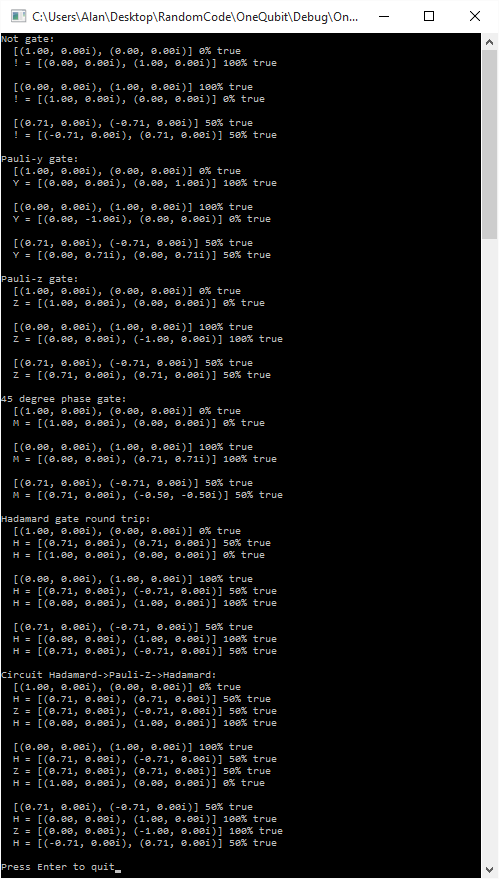
Here’s the output of the program, showing the qubit circuits in action:

Next Up

In the next part, we’ll look at how multiple qubits work together in quantum circuits so we can do more interesting things. We might need a quick post explaining the Bloch sphere before that though. It’s a fairly important thing, but this post is already enough to digest, so I didn’t include it.

Quantum Computing References

I’m in the middle of some research to better understand quantum computing so that I can write a short series of blog posts entitled “Quantum Computing for Programmers”.

These posts will be light on – and possibly completely absent of – hardcore math and physics, and instead speak more to programmers. It will aim to show the rules of quantum computing, explain which operations are fast and which aren’t, show the basic building blocks of quantum logic, combine those simple gates into more complicated quantum circuits, and most importantly it will have simple sample C++ code which shows this stuff in action, so you can do your own (simulated) quantum computing experimentation and exploration on your own computer.

This page is a list of the references I’ve found so far, and I’ll keep updating it as I find new, useful references.