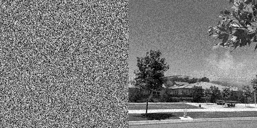
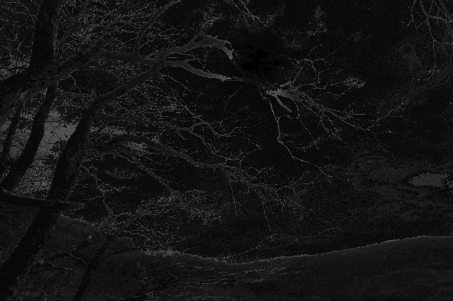
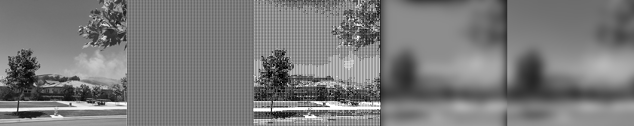
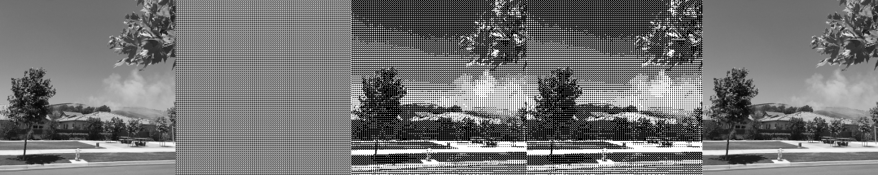
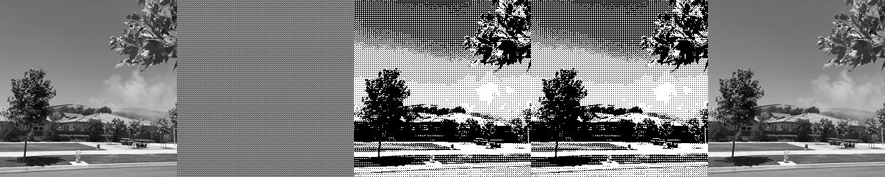
After I put out the last post, Mikkel Gjoel (@pixelmager), made an interesting observation that you can see summarized in his image below. (tweet / thread here)
BTW Mikkel has an amazing presentation about rendering the beautiful game “Inside” that you should check out. Lots of interesting techniques used, including some enlightening uses of noise.
YouTube –
Low Complexity, High Fidelity: The Rendering of INSIDE
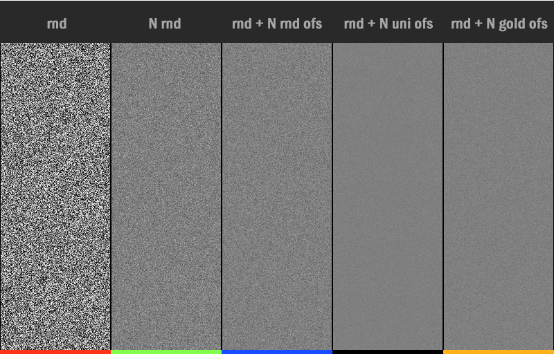
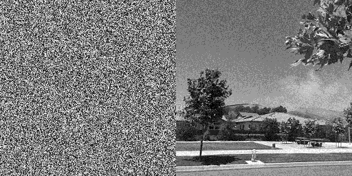
The images left to right are:
- One frame of white noise
- N frames of white noise averaged.
- N frames averaged where the first frame is white noise, and a per frame random number is added to all pixels every frame.
- N frames averaged where the first frame is white noise, and 1/N is added to all pixels every frame.
- N frames averaged where the first frame is white noise, and the golden ratio is added to all pixels every frame.
In the above, the smoother and closer to middle grey that an image is, the better it is – that means it converged to the true result of the integral better.
Surprisingly it looks like adding 1/N outperforms the golden ratio, which means that regular spaced samples are outperforming a low discrepancy sequence!
To compare apples to apples, we’ll do the “golden ratio” tests we did last post, but instead do them with adding this uniform value instead.
To be explicit, there are 8 frames and they are:
- Frame 0: The noise
- Frame 1: The noise + 1/8
- Frame 2: The noise + 2/8
- …
- Frame 7: the noise + 7/8
Modulus is used to keep the values between 0 and 1.
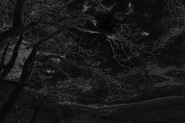
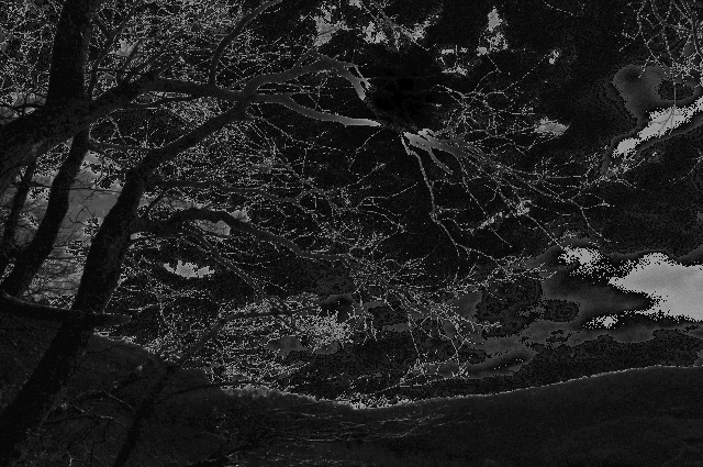
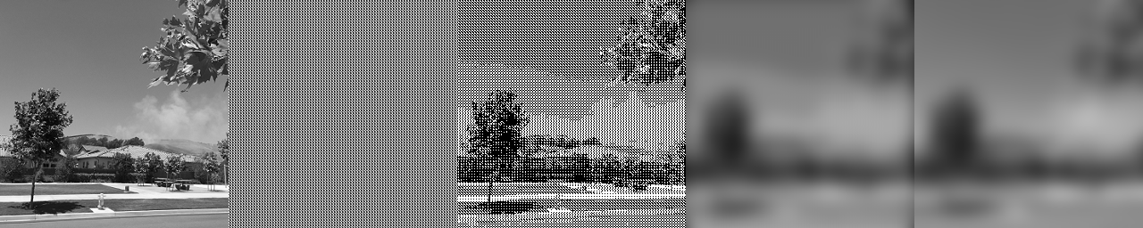
Below is how white noise looks animated with golden ratio (top) vs uniform values (bottom). There are 8 frames and it’s played at 8fps so it loops every second.
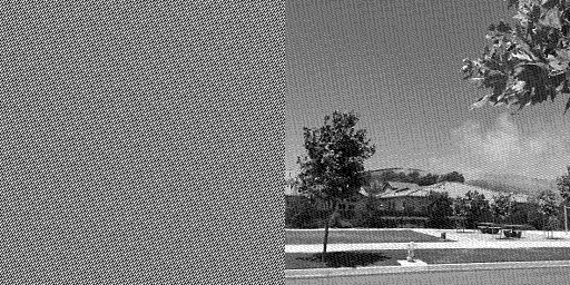
Interleaved Gradient Noise. Top is golden ratio, bottom is uniform.

Blue Noise. Top is golden ratio, bottom is uniform.

The uniform ones look pretty similar. Maybe a little smoother, but it’s hard to tell by just looking at it. Interestingly, the frequency content of the blue noise seems more stable using these uniform values instead of golden ratio.
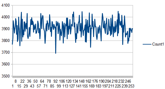
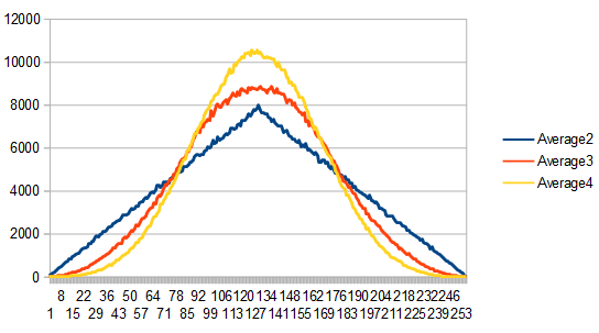
The histogram data of the noise was the same for all frames of animation, just like in last post, which is a good thing. The important bit is that adding a uniform value doesn’t modify the histogram shape, other than changing which counts go to which specific buckets. Ideally the histogram would start out perfectly even like the blue noise does, but since this post is about the “adding uniform values” process, and not about the starting noise, this shows that the process does the right thing with the histogram.
- White Noise – min 213, max 306, average 256, std dev 16.51
- Interleaved Gradient Noise – min 245, max 266, average 256, std dev 2.87
- Blue Noise – min, max, average are 256, std dev 0.
Let’s look at the integrated animations.
White noise. Top is golden ratio, bottom is uniform.
Interleaved gradient noise. Top is golden ratio, bottom is uniform.


Blue noise. Top is golden ratio, bottom is uniform.


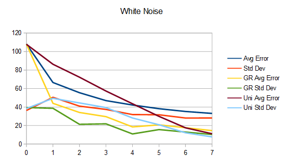
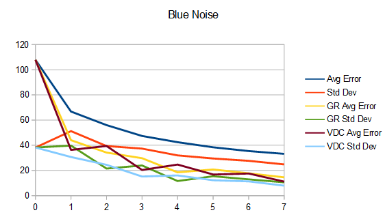
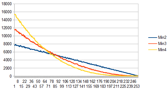
The differences between these animations are subtle unless you know what you are looking for specifically so let’s check out the final frames and the error graphs.
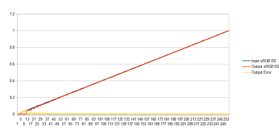
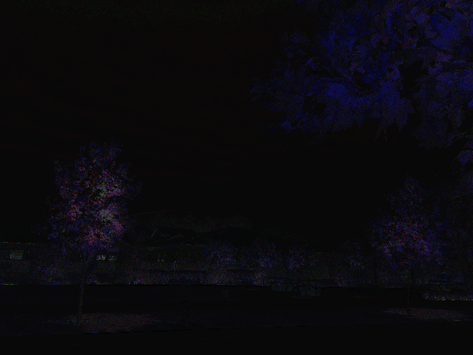
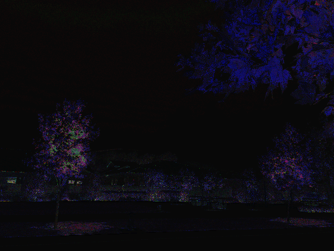
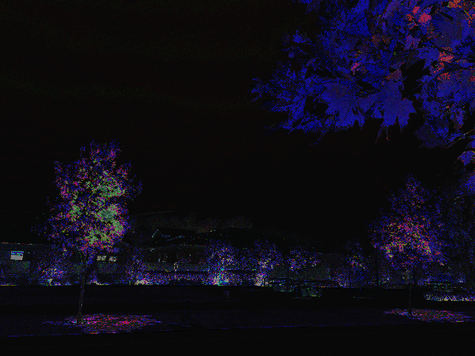
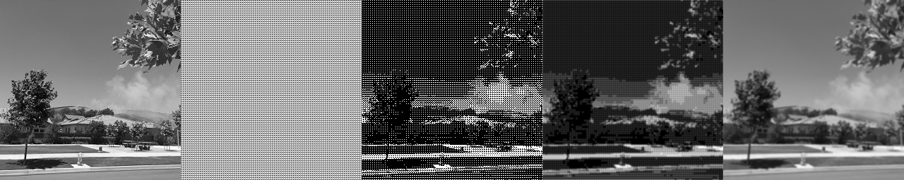
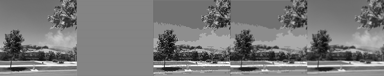
Each noise comparison below has three images. The first image is the “naive” way to animate the noise. The second uses golden ratio instead. The third one uses 1/N. The first two images (and techniques) are from (and explained in) the last post, and the third image is the technique from this post.
White noise. Naive (top), golden ratio (mid), uniform (bottom).

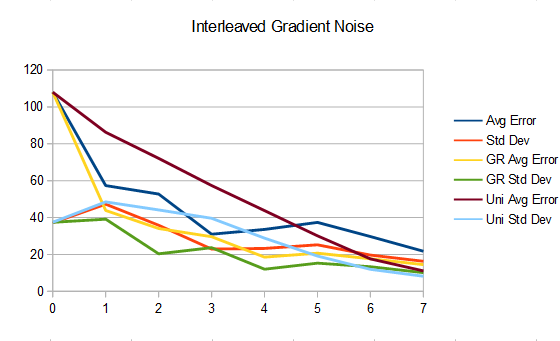
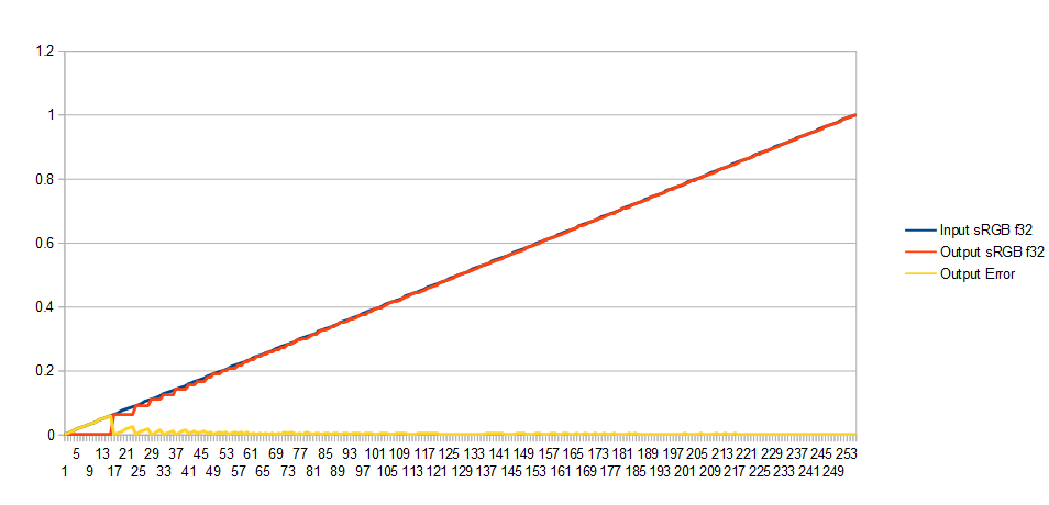
Interleaved gradient noise. Naive (top), golden ratio (mid), uniform (bottom).


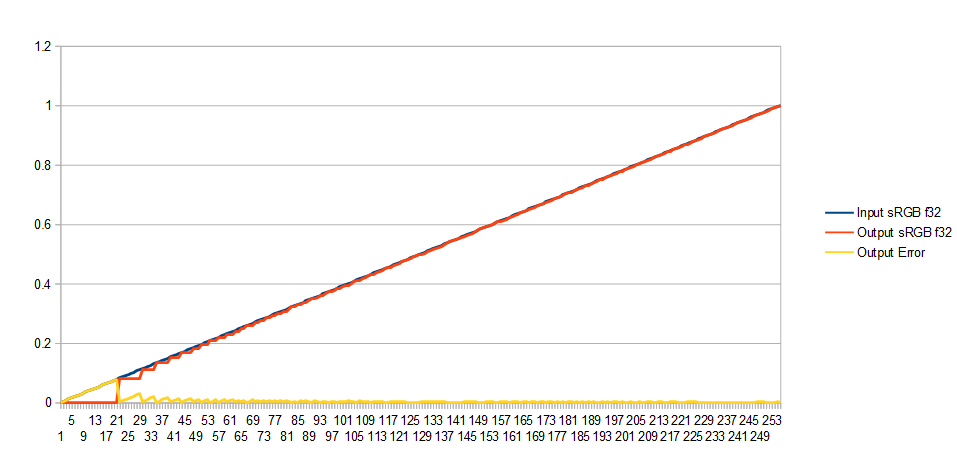
Blue noise. Naive (top), golden ratio (mid), uniform (bottom).


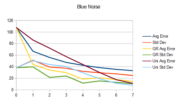
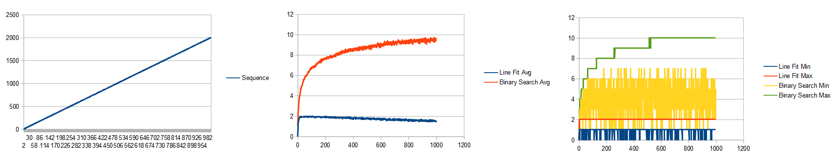
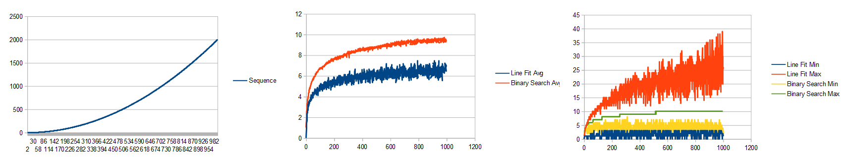
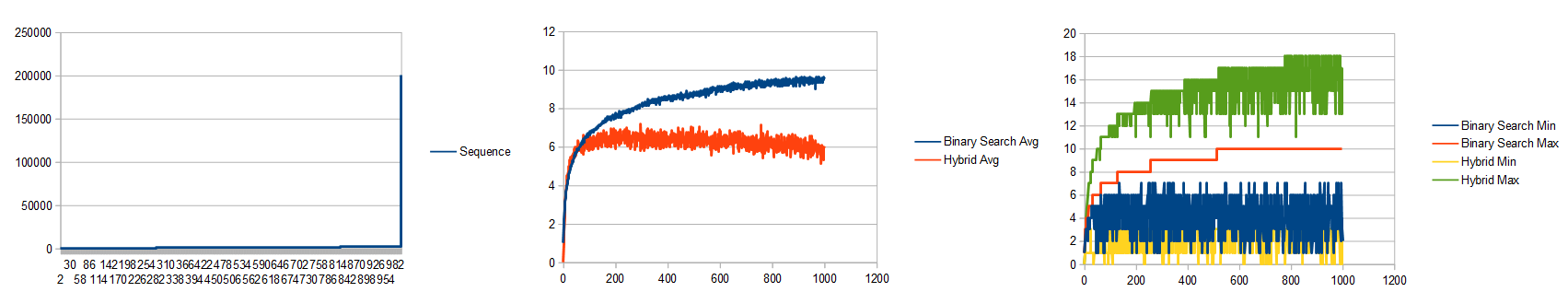
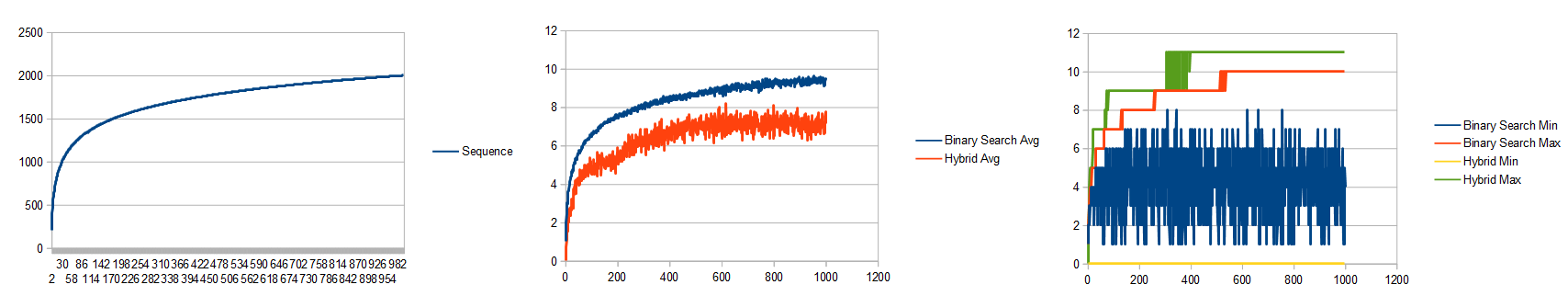
So, what’s interesting is that the uniform sampling over time has lower error and standard deviation (variance) than golden ratio, which has less than the naive method. However, it’s only at the end that the uniform sampling over time has the best results, and it’s actually quite terrible until then.
The reason for this is that uniform has good coverage over the sample space, but it takes until the last frame to get that good coverage because each frame takes a small step over the remaining sample space.
What might work out better would be if our first frame was the normal noise, but then the second frame was the normal noise plus a half, so we get the most information we possibly can from that sample by splitting the sample space in half. We would then want to cut the two halves of the space space in half, and so the next two frames would be the noise plus 1/4 and the noise plus 3/4. We would then continue with 1/8, 5/8, 3/8 and 7/8 (note we didn’t do these 1/8 steps in order. We did it in the order that gives us the most information the most quickly!). At the end of all this, we would have our 8 uniformly spaced samples over time, but we would have taken the samples in an order that makes our intermediate frames look better hopefully.
Now, interestingly, that number sequence I just described has a name. It’s the base 2 Van Der Corput sequence, which is a type of low discrepancy sequence. It’s also the 1D version of the Halton sequence, and is related to other sequences as well. More info here: When Random Numbers Are Too Random: Low Discrepancy Sequences
Mikkel mentioned he thought this would be helpful, and I was thinking the same thing too. Let’s see how it does!
White noise. Uniform (top), Van Der Corput (bottom).
Interleaved gradient noise. Uniform (top), Van Der Corput (bottom).

Blue noise. Uniform (top), Van Der Corput (bottom).

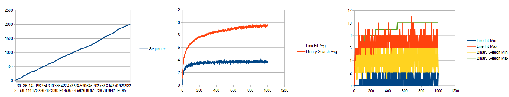
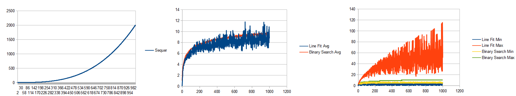
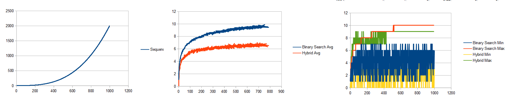
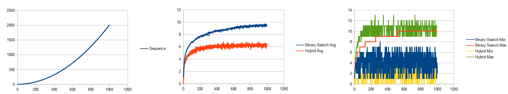
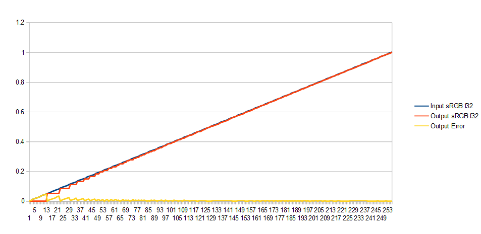
The final frames look the same as before (and the same as each other), so I won’t show those again but here are the updated graphs.
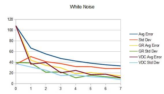
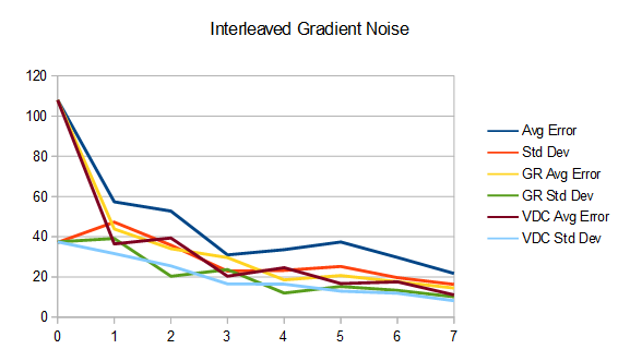
Interestingly, using the Van Der Corput sequence has put intermediate frames more in line with golden ratio, while of course still being superior at the final frame.
I’ve been trying to understand why uniform sampling over time out performs the golden ratio which acts more like blue noise over time. I still don’t grasp why it works as well as it does, but the proof is in the pudding.
Theoretically, this uniform sampling over time should lead to the possibility of aliasing on the time axis, since blue noise / white noise (and other randomness) get rid of the aliasing in exchange for noise.
Noise over the time dimension would mean missing details that were smaller than the sample spacing size. in our case, we are using the time sampled values (noise + uniform value) to threshold a source image to make a sample. It may be that since we are thresholding, that aliasing isn’t possible since our sample represents everything below or equal to the value?
I’m not really sure, but will be thinking about it for a while. If you have any insights please let me know!
It would be interesting to try an actual 1d blue noise sequence and see how it compares. If it does better, it sounds like it would be worth while to try jittering the uniform sampled values on the time axis to try and approximate blue noise a bit. Mikkel tried the jittering and said it gave significantly worse results, so that seems like a no go.
Lastly, some other logical experiments from here seem to be…
- See how other forms of noise and ordered dithers do, including perhaps a Bayer Matrix. IG noise seems to naturally do better on the time axis for some reason I don’t fully understand yet. There may be some interesting properties of other noise waiting to be found.
- Do we get any benefits in this context by arranging the interleaved gradient noise in a spiral like Jorge mentions in his presentation? (Next Generation Post Processing In Call Of Duty: Advanced Warfare
- It would be interesting to see how this works in a more open ended case – such as if you had temporal AA which was averaging a variable number of pixels each frame. Would doing a van Der Corput sequence give good results there? Would you keep track of sample counts per pixel and keep marching the Van Der Corput forward for each pixel individually? Or would you just pick something like an 8 Van Der Corput sequence, adding the current sequence to all pixels and looping that sequence every 8 frames? It really would be interesting to see what is best in that sort of a setup.
I’m sure there are all sorts of other things to try to. This is a deep, interesting and important topic for graphics and beyond (:
Code
Source code below, but it’s also available on github, along with the source images used: Github:
Atrix256/RandomCode/AnimatedNoise
#define _CRT_SECURE_NO_WARNINGS
#include <windows.h> // for bitmap headers. Sorry non windows people!
#include <stdint.h>
#include <vector>
#include <random>
#include <atomic>
#include <thread>
#include <complex>
#include <array>
typedef uint8_t uint8;
const float c_pi = 3.14159265359f;
// settings
const bool c_doDFT = true;
// globals
FILE* g_logFile = nullptr;
//======================================================================================
inline float Lerp (float A, float B, float t)
{
return A * (1.0f - t) + B * t;
}
//======================================================================================
struct SImageData
{
SImageData ()
: m_width(0)
, m_height(0)
{ }
size_t m_width;
size_t m_height;
size_t m_pitch;
std::vector<uint8> m_pixels;
};
//======================================================================================
struct SColor
{
SColor (uint8 _R = 0, uint8 _G = 0, uint8 _B = 0)
: R(_R), G(_G), B(_B)
{ }
inline void Set (uint8 _R, uint8 _G, uint8 _B)
{
R = _R;
G = _G;
B = _B;
}
uint8 B, G, R;
};
//======================================================================================
struct SImageDataComplex
{
SImageDataComplex ()
: m_width(0)
, m_height(0)
{ }
size_t m_width;
size_t m_height;
std::vector<std::complex<float>> m_pixels;
};
//======================================================================================
std::complex<float> DFTPixel (const SImageData &srcImage, size_t K, size_t L)
{
std::complex<float> ret(0.0f, 0.0f);
for (size_t x = 0; x < srcImage.m_width; ++x)
{
for (size_t y = 0; y < srcImage.m_height; ++y)
{
// Get the pixel value (assuming greyscale) and convert it to [0,1] space
const uint8 *src = &srcImage.m_pixels[(y * srcImage.m_pitch) + x * 3];
float grey = float(src[0]) / 255.0f;
// Add to the sum of the return value
float v = float(K * x) / float(srcImage.m_width);
v += float(L * y) / float(srcImage.m_height);
ret += std::complex<float>(grey, 0.0f) * std::polar<float>(1.0f, -2.0f * c_pi * v);
}
}
return ret;
}
//======================================================================================
void ImageDFT (const SImageData &srcImage, SImageDataComplex &destImage)
{
// NOTE: this function assumes srcImage is greyscale, so works on only the red component of srcImage.
// ImageToGrey() will convert an image to greyscale.
// size the output dft data
destImage.m_width = srcImage.m_width;
destImage.m_height = srcImage.m_height;
destImage.m_pixels.resize(destImage.m_width*destImage.m_height);
size_t numThreads = std::thread::hardware_concurrency();
//if (numThreads > 0)
//numThreads = numThreads - 1;
std::vector<std::thread> threads;
threads.resize(numThreads);
printf("Doing DFT with %zu threads...\n", numThreads);
// calculate 2d dft (brute force, not using fast fourier transform) multithreadedly
std::atomic<size_t> nextRow(0);
for (std::thread& t : threads)
{
t = std::thread(
[&] ()
{
size_t row = nextRow.fetch_add(1);
bool reportProgress = (row == 0);
int lastPercent = -1;
while (row < srcImage.m_height)
{
// calculate the DFT for every pixel / frequency in this row
for (size_t x = 0; x < srcImage.m_width; ++x)
{
destImage.m_pixels[row * destImage.m_width + x] = DFTPixel(srcImage, x, row);
}
// report progress if we should
if (reportProgress)
{
int percent = int(100.0f * float(row) / float(srcImage.m_height));
if (lastPercent != percent)
{
lastPercent = percent;
printf(" \rDFT: %i%%", lastPercent);
}
}
// go to the next row
row = nextRow.fetch_add(1);
}
}
);
}
for (std::thread& t : threads)
t.join();
printf("\n");
}
//======================================================================================
void GetMagnitudeData (const SImageDataComplex& srcImage, SImageData& destImage)
{
// size the output image
destImage.m_width = srcImage.m_width;
destImage.m_height = srcImage.m_height;
destImage.m_pitch = 4 * ((srcImage.m_width * 24 + 31) / 32);
destImage.m_pixels.resize(destImage.m_pitch*destImage.m_height);
// get floating point magnitude data
std::vector<float> magArray;
magArray.resize(srcImage.m_width*srcImage.m_height);
float maxmag = 0.0f;
for (size_t x = 0; x < srcImage.m_width; ++x)
{
for (size_t y = 0; y < srcImage.m_height; ++y)
{
// Offset the information by half width & height in the positive direction.
// This makes frequency 0 (DC) be at the image origin, like most diagrams show it.
int k = (x + (int)srcImage.m_width / 2) % (int)srcImage.m_width;
int l = (y + (int)srcImage.m_height / 2) % (int)srcImage.m_height;
const std::complex<float> &src = srcImage.m_pixels[l*srcImage.m_width + k];
float mag = std::abs(src);
if (mag > maxmag)
maxmag = mag;
magArray[y*srcImage.m_width + x] = mag;
}
}
if (maxmag == 0.0f)
maxmag = 1.0f;
const float c = 255.0f / log(1.0f+maxmag);
// normalize the magnitude data and send it back in [0, 255]
for (size_t x = 0; x < srcImage.m_width; ++x)
{
for (size_t y = 0; y < srcImage.m_height; ++y)
{
float src = c * log(1.0f + magArray[y*srcImage.m_width + x]);
uint8 magu8 = uint8(src);
uint8* dest = &destImage.m_pixels[y*destImage.m_pitch + x * 3];
dest[0] = magu8;
dest[1] = magu8;
dest[2] = magu8;
}
}
}
//======================================================================================
bool ImageSave (const SImageData &image, const char *fileName)
{
// open the file if we can
FILE *file;
file = fopen(fileName, "wb");
if (!file) {
printf("Could not save %s\n", fileName);
return false;
}
// make the header info
BITMAPFILEHEADER header;
BITMAPINFOHEADER infoHeader;
header.bfType = 0x4D42;
header.bfReserved1 = 0;
header.bfReserved2 = 0;
header.bfOffBits = 54;
infoHeader.biSize = 40;
infoHeader.biWidth = (LONG)image.m_width;
infoHeader.biHeight = (LONG)image.m_height;
infoHeader.biPlanes = 1;
infoHeader.biBitCount = 24;
infoHeader.biCompression = 0;
infoHeader.biSizeImage = (DWORD) image.m_pixels.size();
infoHeader.biXPelsPerMeter = 0;
infoHeader.biYPelsPerMeter = 0;
infoHeader.biClrUsed = 0;
infoHeader.biClrImportant = 0;
header.bfSize = infoHeader.biSizeImage + header.bfOffBits;
// write the data and close the file
fwrite(&header, sizeof(header), 1, file);
fwrite(&infoHeader, sizeof(infoHeader), 1, file);
fwrite(&image.m_pixels[0], infoHeader.biSizeImage, 1, file);
fclose(file);
return true;
}
//======================================================================================
bool ImageLoad (const char *fileName, SImageData& imageData)
{
// open the file if we can
FILE *file;
file = fopen(fileName, "rb");
if (!file)
return false;
// read the headers if we can
BITMAPFILEHEADER header;
BITMAPINFOHEADER infoHeader;
if (fread(&header, sizeof(header), 1, file) != 1 ||
fread(&infoHeader, sizeof(infoHeader), 1, file) != 1 ||
header.bfType != 0x4D42 || infoHeader.biBitCount != 24)
{
fclose(file);
return false;
}
// read in our pixel data if we can. Note that it's in BGR order, and width is padded to the next power of 4
imageData.m_pixels.resize(infoHeader.biSizeImage);
fseek(file, header.bfOffBits, SEEK_SET);
if (fread(&imageData.m_pixels[0], imageData.m_pixels.size(), 1, file) != 1)
{
fclose(file);
return false;
}
imageData.m_width = infoHeader.biWidth;
imageData.m_height = infoHeader.biHeight;
imageData.m_pitch = 4 * ((imageData.m_width * 24 + 31) / 32);
fclose(file);
return true;
}
//======================================================================================
void ImageInit (SImageData& image, size_t width, size_t height)
{
image.m_width = width;
image.m_height = height;
image.m_pitch = 4 * ((width * 24 + 31) / 32);
image.m_pixels.resize(image.m_pitch * image.m_height);
std::fill(image.m_pixels.begin(), image.m_pixels.end(), 0);
}
//======================================================================================
template <typename LAMBDA>
void ImageForEachPixel (SImageData& image, const LAMBDA& lambda)
{
size_t pixelIndex = 0;
for (size_t y = 0; y < image.m_height; ++y)
{
SColor* pixel = (SColor*)&image.m_pixels[y * image.m_pitch];
for (size_t x = 0; x < image.m_width; ++x)
{
lambda(*pixel, pixelIndex);
++pixel;
++pixelIndex;
}
}
}
//======================================================================================
template <typename LAMBDA>
void ImageForEachPixel (const SImageData& image, const LAMBDA& lambda)
{
size_t pixelIndex = 0;
for (size_t y = 0; y < image.m_height; ++y)
{
SColor* pixel = (SColor*)&image.m_pixels[y * image.m_pitch];
for (size_t x = 0; x < image.m_width; ++x)
{
lambda(*pixel, pixelIndex);
++pixel;
++pixelIndex;
}
}
}
//======================================================================================
void ImageConvertToLuma (SImageData& image)
{
ImageForEachPixel(
image,
[] (SColor& pixel, size_t pixelIndex)
{
float luma = float(pixel.R) * 0.3f + float(pixel.G) * 0.59f + float(pixel.B) * 0.11f;
uint8 lumau8 = uint8(luma + 0.5f);
pixel.R = lumau8;
pixel.G = lumau8;
pixel.B = lumau8;
}
);
}
//======================================================================================
void ImageCombine2 (const SImageData& imageA, const SImageData& imageB, SImageData& result)
{
// put the images side by side. A on left, B on right
ImageInit(result, imageA.m_width + imageB.m_width, max(imageA.m_height, imageB.m_height));
std::fill(result.m_pixels.begin(), result.m_pixels.end(), 0);
// image A on left
for (size_t y = 0; y < imageA.m_height; ++y)
{
SColor* destPixel = (SColor*)&result.m_pixels[y * result.m_pitch];
SColor* srcPixel = (SColor*)&imageA.m_pixels[y * imageA.m_pitch];
for (size_t x = 0; x < imageA.m_width; ++x)
{
destPixel[0] = srcPixel[0];
++destPixel;
++srcPixel;
}
}
// image B on right
for (size_t y = 0; y < imageB.m_height; ++y)
{
SColor* destPixel = (SColor*)&result.m_pixels[y * result.m_pitch + imageA.m_width * 3];
SColor* srcPixel = (SColor*)&imageB.m_pixels[y * imageB.m_pitch];
for (size_t x = 0; x < imageB.m_width; ++x)
{
destPixel[0] = srcPixel[0];
++destPixel;
++srcPixel;
}
}
}
//======================================================================================
void ImageCombine3 (const SImageData& imageA, const SImageData& imageB, const SImageData& imageC, SImageData& result)
{
// put the images side by side. A on left, B in middle, C on right
ImageInit(result, imageA.m_width + imageB.m_width + imageC.m_width, max(max(imageA.m_height, imageB.m_height), imageC.m_height));
std::fill(result.m_pixels.begin(), result.m_pixels.end(), 0);
// image A on left
for (size_t y = 0; y < imageA.m_height; ++y)
{
SColor* destPixel = (SColor*)&result.m_pixels[y * result.m_pitch];
SColor* srcPixel = (SColor*)&imageA.m_pixels[y * imageA.m_pitch];
for (size_t x = 0; x < imageA.m_width; ++x)
{
destPixel[0] = srcPixel[0];
++destPixel;
++srcPixel;
}
}
// image B in middle
for (size_t y = 0; y < imageB.m_height; ++y)
{
SColor* destPixel = (SColor*)&result.m_pixels[y * result.m_pitch + imageA.m_width * 3];
SColor* srcPixel = (SColor*)&imageB.m_pixels[y * imageB.m_pitch];
for (size_t x = 0; x < imageB.m_width; ++x)
{
destPixel[0] = srcPixel[0];
++destPixel;
++srcPixel;
}
}
// image C on right
for (size_t y = 0; y < imageC.m_height; ++y)
{
SColor* destPixel = (SColor*)&result.m_pixels[y * result.m_pitch + imageA.m_width * 3 + imageC.m_width * 3];
SColor* srcPixel = (SColor*)&imageC.m_pixels[y * imageC.m_pitch];
for (size_t x = 0; x < imageC.m_width; ++x)
{
destPixel[0] = srcPixel[0];
++destPixel;
++srcPixel;
}
}
}
//======================================================================================
float GoldenRatioMultiple (size_t multiple)
{
return float(multiple) * (1.0f + std::sqrtf(5.0f)) / 2.0f;
}
//======================================================================================
void IntegrationTest (const SImageData& dither, const SImageData& groundTruth, size_t frameIndex, const char* label)
{
// calculate min, max, total and average error
size_t minError = 0;
size_t maxError = 0;
size_t totalError = 0;
size_t pixelCount = 0;
for (size_t y = 0; y < dither.m_height; ++y)
{
SColor* ditherPixel = (SColor*)&dither.m_pixels[y * dither.m_pitch];
SColor* truthPixel = (SColor*)&groundTruth.m_pixels[y * groundTruth.m_pitch];
for (size_t x = 0; x < dither.m_width; ++x)
{
size_t error = 0;
if (ditherPixel->R > truthPixel->R)
error = ditherPixel->R - truthPixel->R;
else
error = truthPixel->R - ditherPixel->R;
totalError += error;
if ((x == 0 && y == 0) || error < minError)
minError = error;
if ((x == 0 && y == 0) || error > maxError)
maxError = error;
++ditherPixel;
++truthPixel;
++pixelCount;
}
}
float averageError = float(totalError) / float(pixelCount);
// calculate standard deviation
float sumSquaredDiff = 0.0f;
for (size_t y = 0; y < dither.m_height; ++y)
{
SColor* ditherPixel = (SColor*)&dither.m_pixels[y * dither.m_pitch];
SColor* truthPixel = (SColor*)&groundTruth.m_pixels[y * groundTruth.m_pitch];
for (size_t x = 0; x < dither.m_width; ++x)
{
size_t error = 0;
if (ditherPixel->R > truthPixel->R)
error = ditherPixel->R - truthPixel->R;
else
error = truthPixel->R - ditherPixel->R;
float diff = float(error) - averageError;
sumSquaredDiff += diff*diff;
}
}
float stdDev = std::sqrtf(sumSquaredDiff / float(pixelCount - 1));
// report results
fprintf(g_logFile, "%s %zu error\n", label, frameIndex);
fprintf(g_logFile, " min error: %zu\n", minError);
fprintf(g_logFile, " max error: %zu\n", maxError);
fprintf(g_logFile, " avg error: %0.2f\n", averageError);
fprintf(g_logFile, " stddev: %0.2f\n", stdDev);
fprintf(g_logFile, "\n");
}
//======================================================================================
void HistogramTest (const SImageData& noise, size_t frameIndex, const char* label)
{
std::array<size_t, 256> counts;
std::fill(counts.begin(), counts.end(), 0);
ImageForEachPixel(
noise,
[&] (const SColor& pixel, size_t pixelIndex)
{
counts[pixel.R]++;
}
);
// calculate min, max, total and average
size_t minCount = 0;
size_t maxCount = 0;
size_t totalCount = 0;
for (size_t i = 0; i < 256; ++i)
{
if (i == 0 || counts[i] < minCount)
minCount = counts[i];
if (i == 0 || counts[i] > maxCount)
maxCount = counts[i];
totalCount += counts[i];
}
float averageCount = float(totalCount) / float(256.0f);
// calculate standard deviation
float sumSquaredDiff = 0.0f;
for (size_t i = 0; i < 256; ++i)
{
float diff = float(counts[i]) - averageCount;
sumSquaredDiff += diff*diff;
}
float stdDev = std::sqrtf(sumSquaredDiff / 255.0f);
// report results
fprintf(g_logFile, "%s %zu histogram\n", label, frameIndex);
fprintf(g_logFile, " min count: %zu\n", minCount);
fprintf(g_logFile, " max count: %zu\n", maxCount);
fprintf(g_logFile, " avg count: %0.2f\n", averageCount);
fprintf(g_logFile, " stddev: %0.2f\n", stdDev);
fprintf(g_logFile, " counts: ");
for (size_t i = 0; i < 256; ++i)
{
if (i > 0)
fprintf(g_logFile, ", ");
fprintf(g_logFile, "%zu", counts[i]);
}
fprintf(g_logFile, "\n\n");
}
//======================================================================================
void GenerateWhiteNoise (SImageData& image, size_t width, size_t height)
{
ImageInit(image, width, height);
std::random_device rd;
std::mt19937 rng(rd());
std::uniform_int_distribution<unsigned int> dist(0, 255);
ImageForEachPixel(
image,
[&] (SColor& pixel, size_t pixelIndex)
{
uint8 value = dist(rng);
pixel.R = value;
pixel.G = value;
pixel.B = value;
}
);
}
//======================================================================================
void GenerateInterleavedGradientNoise (SImageData& image, size_t width, size_t height, float offsetX, float offsetY)
{
ImageInit(image, width, height);
std::random_device rd;
std::mt19937 rng(rd());
std::uniform_int_distribution<unsigned int> dist(0, 255);
for (size_t y = 0; y < height; ++y)
{
SColor* pixel = (SColor*)&image.m_pixels[y * image.m_pitch];
for (size_t x = 0; x < width; ++x)
{
float valueFloat = std::fmodf(52.9829189f * std::fmod(0.06711056f*float(x + offsetX) + 0.00583715f*float(y + offsetY), 1.0f), 1.0f);
size_t valueBig = size_t(valueFloat * 256.0f);
uint8 value = uint8(valueBig % 256);
pixel->R = value;
pixel->G = value;
pixel->B = value;
++pixel;
}
}
}
//======================================================================================
template <size_t NUM_SAMPLES>
void GenerateVanDerCoruptSequence (std::array<float, NUM_SAMPLES>& samples, size_t base)
{
for (size_t i = 0; i < NUM_SAMPLES; ++i)
{
samples[i] = 0.0f;
float denominator = float(base);
size_t n = i;
while (n > 0)
{
size_t multiplier = n % base;
samples[i] += float(multiplier) / denominator;
n = n / base;
denominator *= base;
}
}
}
//======================================================================================
void DitherWithTexture (const SImageData& ditherImage, const SImageData& noiseImage, SImageData& result)
{
// init the result image
ImageInit(result, ditherImage.m_width, ditherImage.m_height);
// make the result image
for (size_t y = 0; y < ditherImage.m_height; ++y)
{
SColor* srcDitherPixel = (SColor*)&ditherImage.m_pixels[y * ditherImage.m_pitch];
SColor* destDitherPixel = (SColor*)&result.m_pixels[y * result.m_pitch];
for (size_t x = 0; x < ditherImage.m_width; ++x)
{
// tile the noise in case it isn't the same size as the image we are dithering
size_t noiseX = x % noiseImage.m_width;
size_t noiseY = y % noiseImage.m_height;
SColor* noisePixel = (SColor*)&noiseImage.m_pixels[noiseY * noiseImage.m_pitch + noiseX * 3];
uint8 value = 0;
if (noisePixel->R < srcDitherPixel->R)
value = 255;
destDitherPixel->R = value;
destDitherPixel->G = value;
destDitherPixel->B = value;
++srcDitherPixel;
++destDitherPixel;
}
}
}
//======================================================================================
void DitherWhiteNoise (const SImageData& ditherImage)
{
printf("\n%s\n", __FUNCTION__);
// make noise
SImageData noise;
GenerateWhiteNoise(noise, ditherImage.m_width, ditherImage.m_height);
// dither the image
SImageData dither;
DitherWithTexture(ditherImage, noise, dither);
// save the results
SImageData combined;
ImageCombine3(ditherImage, noise, dither, combined);
ImageSave(combined, "out/still_whitenoise.bmp");
}
//======================================================================================
void DitherInterleavedGradientNoise (const SImageData& ditherImage)
{
printf("\n%s\n", __FUNCTION__);
// make noise
SImageData noise;
GenerateInterleavedGradientNoise(noise, ditherImage.m_width, ditherImage.m_height, 0.0f, 0.0f);
// dither the image
SImageData dither;
DitherWithTexture(ditherImage, noise, dither);
// save the results
SImageData combined;
ImageCombine3(ditherImage, noise, dither, combined);
ImageSave(combined, "out/still_ignoise.bmp");
}
//======================================================================================
void DitherBlueNoise (const SImageData& ditherImage, const SImageData& blueNoise)
{
printf("\n%s\n", __FUNCTION__);
// dither the image
SImageData dither;
DitherWithTexture(ditherImage, blueNoise, dither);
// save the results
SImageData combined;
ImageCombine3(ditherImage, blueNoise, dither, combined);
ImageSave(combined, "out/still_bluenoise.bmp");
}
//======================================================================================
void DitherWhiteNoiseAnimated (const SImageData& ditherImage)
{
printf("\n%s\n", __FUNCTION__);
// animate 8 frames
for (size_t i = 0; i < 8; ++i)
{
char fileName[256];
sprintf(fileName, "out/anim_whitenoise%zu.bmp", i);
// make noise
SImageData noise;
GenerateWhiteNoise(noise, ditherImage.m_width, ditherImage.m_height);
// dither the image
SImageData dither;
DitherWithTexture(ditherImage, noise, dither);
// save the results
SImageData combined;
ImageCombine2(noise, dither, combined);
ImageSave(combined, fileName);
}
}
//======================================================================================
void DitherInterleavedGradientNoiseAnimated (const SImageData& ditherImage)
{
printf("\n%s\n", __FUNCTION__);
std::random_device rd;
std::mt19937 rng(rd());
std::uniform_real_distribution<float> dist(0.0f, 1000.0f);
// animate 8 frames
for (size_t i = 0; i < 8; ++i)
{
char fileName[256];
sprintf(fileName, "out/anim_ignoise%zu.bmp", i);
// make noise
SImageData noise;
GenerateInterleavedGradientNoise(noise, ditherImage.m_width, ditherImage.m_height, dist(rng), dist(rng));
// dither the image
SImageData dither;
DitherWithTexture(ditherImage, noise, dither);
// save the results
SImageData combined;
ImageCombine2(noise, dither, combined);
ImageSave(combined, fileName);
}
}
//======================================================================================
void DitherBlueNoiseAnimated (const SImageData& ditherImage, const SImageData blueNoise[8])
{
printf("\n%s\n", __FUNCTION__);
// animate 8 frames
for (size_t i = 0; i < 8; ++i)
{
char fileName[256];
sprintf(fileName, "out/anim_bluenoise%zu.bmp", i);
// dither the image
SImageData dither;
DitherWithTexture(ditherImage, blueNoise[i], dither);
// save the results
SImageData combined;
ImageCombine2(blueNoise[i], dither, combined);
ImageSave(combined, fileName);
}
}
//======================================================================================
void DitherWhiteNoiseAnimatedIntegrated (const SImageData& ditherImage)
{
printf("\n%s\n", __FUNCTION__);
std::vector<float> integration;
integration.resize(ditherImage.m_width * ditherImage.m_height);
std::fill(integration.begin(), integration.end(), 0.0f);
// animate 8 frames
for (size_t i = 0; i < 8; ++i)
{
char fileName[256];
sprintf(fileName, "out/animint_whitenoise%zu.bmp", i);
// make noise
SImageData noise;
GenerateWhiteNoise(noise, ditherImage.m_width, ditherImage.m_height);
// dither the image
SImageData dither;
DitherWithTexture(ditherImage, noise, dither);
// integrate and put the current integration results into the dither image
ImageForEachPixel(
dither,
[&] (SColor& pixel, size_t pixelIndex)
{
float pixelValueFloat = float(pixel.R) / 255.0f;
integration[pixelIndex] = Lerp(integration[pixelIndex], pixelValueFloat, 1.0f / float(i+1));
uint8 integratedPixelValue = uint8(integration[pixelIndex] * 255.0f);
pixel.R = integratedPixelValue;
pixel.G = integratedPixelValue;
pixel.B = integratedPixelValue;
}
);
// do an integration test
IntegrationTest(dither, ditherImage, i, __FUNCTION__);
// save the results
SImageData combined;
ImageCombine2(noise, dither, combined);
ImageSave(combined, fileName);
}
}
//======================================================================================
void DitherInterleavedGradientNoiseAnimatedIntegrated (const SImageData& ditherImage)
{
printf("\n%s\n", __FUNCTION__);
std::vector<float> integration;
integration.resize(ditherImage.m_width * ditherImage.m_height);
std::fill(integration.begin(), integration.end(), 0.0f);
std::random_device rd;
std::mt19937 rng(rd());
std::uniform_real_distribution<float> dist(0.0f, 1000.0f);
// animate 8 frames
for (size_t i = 0; i < 8; ++i)
{
char fileName[256];
sprintf(fileName, "out/animint_ignoise%zu.bmp", i);
// make noise
SImageData noise;
GenerateInterleavedGradientNoise(noise, ditherImage.m_width, ditherImage.m_height, dist(rng), dist(rng));
// dither the image
SImageData dither;
DitherWithTexture(ditherImage, noise, dither);
// integrate and put the current integration results into the dither image
ImageForEachPixel(
dither,
[&](SColor& pixel, size_t pixelIndex)
{
float pixelValueFloat = float(pixel.R) / 255.0f;
integration[pixelIndex] = Lerp(integration[pixelIndex], pixelValueFloat, 1.0f / float(i + 1));
uint8 integratedPixelValue = uint8(integration[pixelIndex] * 255.0f);
pixel.R = integratedPixelValue;
pixel.G = integratedPixelValue;
pixel.B = integratedPixelValue;
}
);
// do an integration test
IntegrationTest(dither, ditherImage, i, __FUNCTION__);
// save the results
SImageData combined;
ImageCombine2(noise, dither, combined);
ImageSave(combined, fileName);
}
}
//======================================================================================
void DitherBlueNoiseAnimatedIntegrated (const SImageData& ditherImage, const SImageData blueNoise[8])
{
printf("\n%s\n", __FUNCTION__);
std::vector<float> integration;
integration.resize(ditherImage.m_width * ditherImage.m_height);
std::fill(integration.begin(), integration.end(), 0.0f);
// animate 8 frames
for (size_t i = 0; i < 8; ++i)
{
char fileName[256];
sprintf(fileName, "out/animint_bluenoise%zu.bmp", i);
// dither the image
SImageData dither;
DitherWithTexture(ditherImage, blueNoise[i], dither);
// integrate and put the current integration results into the dither image
ImageForEachPixel(
dither,
[&] (SColor& pixel, size_t pixelIndex)
{
float pixelValueFloat = float(pixel.R) / 255.0f;
integration[pixelIndex] = Lerp(integration[pixelIndex], pixelValueFloat, 1.0f / float(i+1));
uint8 integratedPixelValue = uint8(integration[pixelIndex] * 255.0f);
pixel.R = integratedPixelValue;
pixel.G = integratedPixelValue;
pixel.B = integratedPixelValue;
}
);
// do an integration test
IntegrationTest(dither, ditherImage, i, __FUNCTION__);
// save the results
SImageData combined;
ImageCombine2(blueNoise[i], dither, combined);
ImageSave(combined, fileName);
}
}
//======================================================================================
void DitherWhiteNoiseAnimatedGoldenRatio (const SImageData& ditherImage)
{
printf("\n%s\n", __FUNCTION__);
// make noise
SImageData noiseSrc;
GenerateWhiteNoise(noiseSrc, ditherImage.m_width, ditherImage.m_height);
SImageData noise;
ImageInit(noise, noiseSrc.m_width, noiseSrc.m_height);
SImageDataComplex noiseDFT;
SImageData noiseDFTMag;
// animate 8 frames
for (size_t i = 0; i < 8; ++i)
{
char fileName[256];
sprintf(fileName, "out/animgr_whitenoise%zu.bmp", i);
// add golden ratio to the noise after each frame
noise.m_pixels = noiseSrc.m_pixels;
float add = GoldenRatioMultiple(i);
ImageForEachPixel(
noise,
[&] (SColor& pixel, size_t pixelIndex)
{
float valueFloat = (float(pixel.R) / 255.0f) + add;
size_t valueBig = size_t(valueFloat * 255.0f);
uint8 value = uint8(valueBig % 256);
pixel.R = value;
pixel.G = value;
pixel.B = value;
}
);
// DFT the noise
if (c_doDFT)
{
ImageDFT(noise, noiseDFT);
GetMagnitudeData(noiseDFT, noiseDFTMag);
}
else
{
ImageInit(noiseDFTMag, noise.m_width, noise.m_height);
std::fill(noiseDFTMag.m_pixels.begin(), noiseDFTMag.m_pixels.end(), 0);
}
// Histogram test the noise
HistogramTest(noise, i, __FUNCTION__);
// dither the image
SImageData dither;
DitherWithTexture(ditherImage, noise, dither);
// save the results
SImageData combined;
ImageCombine3(noiseDFTMag, noise, dither, combined);
ImageSave(combined, fileName);
}
}
//======================================================================================
void DitherInterleavedGradientNoiseAnimatedGoldenRatio (const SImageData& ditherImage)
{
printf("\n%s\n", __FUNCTION__);
// make noise
SImageData noiseSrc;
GenerateInterleavedGradientNoise(noiseSrc, ditherImage.m_width, ditherImage.m_height, 0.0f, 0.0f);
SImageData noise;
ImageInit(noise, noiseSrc.m_width, noiseSrc.m_height);
SImageDataComplex noiseDFT;
SImageData noiseDFTMag;
// animate 8 frames
for (size_t i = 0; i < 8; ++i)
{
char fileName[256];
sprintf(fileName, "out/animgr_ignoise%zu.bmp", i);
// add golden ratio to the noise after each frame
noise.m_pixels = noiseSrc.m_pixels;
float add = GoldenRatioMultiple(i);
ImageForEachPixel(
noise,
[&] (SColor& pixel, size_t pixelIndex)
{
float valueFloat = (float(pixel.R) / 255.0f) + add;
size_t valueBig = size_t(valueFloat * 255.0f);
uint8 value = uint8(valueBig % 256);
pixel.R = value;
pixel.G = value;
pixel.B = value;
}
);
// DFT the noise
if (c_doDFT)
{
ImageDFT(noise, noiseDFT);
GetMagnitudeData(noiseDFT, noiseDFTMag);
}
else
{
ImageInit(noiseDFTMag, noise.m_width, noise.m_height);
std::fill(noiseDFTMag.m_pixels.begin(), noiseDFTMag.m_pixels.end(), 0);
}
// Histogram test the noise
HistogramTest(noise, i, __FUNCTION__);
// dither the image
SImageData dither;
DitherWithTexture(ditherImage, noise, dither);
// save the results
SImageData combined;
ImageCombine3(noiseDFTMag, noise, dither, combined);
ImageSave(combined, fileName);
}
}
//======================================================================================
void DitherBlueNoiseAnimatedGoldenRatio (const SImageData& ditherImage, const SImageData& noiseSrc)
{
printf("\n%s\n", __FUNCTION__);
SImageData noise;
ImageInit(noise, noiseSrc.m_width, noiseSrc.m_height);
SImageDataComplex noiseDFT;
SImageData noiseDFTMag;
// animate 8 frames
for (size_t i = 0; i < 8; ++i)
{
char fileName[256];
sprintf(fileName, "out/animgr_bluenoise%zu.bmp", i);
// add golden ratio to the noise after each frame
noise.m_pixels = noiseSrc.m_pixels;
float add = GoldenRatioMultiple(i);
ImageForEachPixel(
noise,
[&] (SColor& pixel, size_t pixelIndex)
{
float valueFloat = (float(pixel.R) / 255.0f) + add;
size_t valueBig = size_t(valueFloat * 255.0f);
uint8 value = uint8(valueBig % 256);
pixel.R = value;
pixel.G = value;
pixel.B = value;
}
);
// DFT the noise
if (c_doDFT)
{
ImageDFT(noise, noiseDFT);
GetMagnitudeData(noiseDFT, noiseDFTMag);
}
else
{
ImageInit(noiseDFTMag, noise.m_width, noise.m_height);
std::fill(noiseDFTMag.m_pixels.begin(), noiseDFTMag.m_pixels.end(), 0);
}
// Histogram test the noise
HistogramTest(noise, i, __FUNCTION__);
// dither the image
SImageData dither;
DitherWithTexture(ditherImage, noise, dither);
// save the results
SImageData combined;
ImageCombine3(noiseDFTMag, noise, dither, combined);
ImageSave(combined, fileName);
}
}
//======================================================================================
void DitherWhiteNoiseAnimatedUniform (const SImageData& ditherImage)
{
printf("\n%s\n", __FUNCTION__);
// make noise
SImageData noiseSrc;
GenerateWhiteNoise(noiseSrc, ditherImage.m_width, ditherImage.m_height);
SImageData noise;
ImageInit(noise, noiseSrc.m_width, noiseSrc.m_height);
SImageDataComplex noiseDFT;
SImageData noiseDFTMag;
// animate 8 frames
for (size_t i = 0; i < 8; ++i)
{
char fileName[256];
sprintf(fileName, "out/animuni_whitenoise%zu.bmp", i);
// add uniform value to the noise after each frame
noise.m_pixels = noiseSrc.m_pixels;
float add = float(i) / 8.0f;
ImageForEachPixel(
noise,
[&] (SColor& pixel, size_t pixelIndex)
{
float valueFloat = (float(pixel.R) / 255.0f) + add;
size_t valueBig = size_t(valueFloat * 255.0f);
uint8 value = uint8(valueBig % 256);
pixel.R = value;
pixel.G = value;
pixel.B = value;
}
);
// DFT the noise
if (c_doDFT)
{
ImageDFT(noise, noiseDFT);
GetMagnitudeData(noiseDFT, noiseDFTMag);
}
else
{
ImageInit(noiseDFTMag, noise.m_width, noise.m_height);
std::fill(noiseDFTMag.m_pixels.begin(), noiseDFTMag.m_pixels.end(), 0);
}
// Histogram test the noise
HistogramTest(noise, i, __FUNCTION__);
// dither the image
SImageData dither;
DitherWithTexture(ditherImage, noise, dither);
// save the results
SImageData combined;
ImageCombine3(noiseDFTMag, noise, dither, combined);
ImageSave(combined, fileName);
}
}
//======================================================================================
void DitherInterleavedGradientNoiseAnimatedUniform (const SImageData& ditherImage)
{
printf("\n%s\n", __FUNCTION__);
// make noise
SImageData noiseSrc;
GenerateInterleavedGradientNoise(noiseSrc, ditherImage.m_width, ditherImage.m_height, 0.0f, 0.0f);
SImageData noise;
ImageInit(noise, noiseSrc.m_width, noiseSrc.m_height);
SImageDataComplex noiseDFT;
SImageData noiseDFTMag;
// animate 8 frames
for (size_t i = 0; i < 8; ++i)
{
char fileName[256];
sprintf(fileName, "out/animuni_ignoise%zu.bmp", i);
// add uniform value to the noise after each frame
noise.m_pixels = noiseSrc.m_pixels;
float add = float(i) / 8.0f;
ImageForEachPixel(
noise,
[&] (SColor& pixel, size_t pixelIndex)
{
float valueFloat = (float(pixel.R) / 255.0f) + add;
size_t valueBig = size_t(valueFloat * 255.0f);
uint8 value = uint8(valueBig % 256);
pixel.R = value;
pixel.G = value;
pixel.B = value;
}
);
// DFT the noise
if (c_doDFT)
{
ImageDFT(noise, noiseDFT);
GetMagnitudeData(noiseDFT, noiseDFTMag);
}
else
{
ImageInit(noiseDFTMag, noise.m_width, noise.m_height);
std::fill(noiseDFTMag.m_pixels.begin(), noiseDFTMag.m_pixels.end(), 0);
}
// Histogram test the noise
HistogramTest(noise, i, __FUNCTION__);
// dither the image
SImageData dither;
DitherWithTexture(ditherImage, noise, dither);
// save the results
SImageData combined;
ImageCombine3(noiseDFTMag, noise, dither, combined);
ImageSave(combined, fileName);
}
}
//======================================================================================
void DitherBlueNoiseAnimatedUniform (const SImageData& ditherImage, const SImageData& noiseSrc)
{
printf("\n%s\n", __FUNCTION__);
SImageData noise;
ImageInit(noise, noiseSrc.m_width, noiseSrc.m_height);
SImageDataComplex noiseDFT;
SImageData noiseDFTMag;
// animate 8 frames
for (size_t i = 0; i < 8; ++i)
{
char fileName[256];
sprintf(fileName, "out/animuni_bluenoise%zu.bmp", i);
// add uniform value to the noise after each frame
noise.m_pixels = noiseSrc.m_pixels;
float add = float(i) / 8.0f;
ImageForEachPixel(
noise,
[&] (SColor& pixel, size_t pixelIndex)
{
float valueFloat = (float(pixel.R) / 255.0f) + add;
size_t valueBig = size_t(valueFloat * 255.0f);
uint8 value = uint8(valueBig % 256);
pixel.R = value;
pixel.G = value;
pixel.B = value;
}
);
// DFT the noise
if (c_doDFT)
{
ImageDFT(noise, noiseDFT);
GetMagnitudeData(noiseDFT, noiseDFTMag);
}
else
{
ImageInit(noiseDFTMag, noise.m_width, noise.m_height);
std::fill(noiseDFTMag.m_pixels.begin(), noiseDFTMag.m_pixels.end(), 0);
}
// Histogram test the noise
HistogramTest(noise, i, __FUNCTION__);
// dither the image
SImageData dither;
DitherWithTexture(ditherImage, noise, dither);
// save the results
SImageData combined;
ImageCombine3(noiseDFTMag, noise, dither, combined);
ImageSave(combined, fileName);
}
}
//======================================================================================
void DitherWhiteNoiseAnimatedGoldenRatioIntegrated (const SImageData& ditherImage)
{
printf("\n%s\n", __FUNCTION__);
std::vector<float> integration;
integration.resize(ditherImage.m_width * ditherImage.m_height);
std::fill(integration.begin(), integration.end(), 0.0f);
// make noise
SImageData noiseSrc;
GenerateWhiteNoise(noiseSrc, ditherImage.m_width, ditherImage.m_height);
SImageData noise;
ImageInit(noise, noiseSrc.m_width, noiseSrc.m_height);
// animate 8 frames
for (size_t i = 0; i < 8; ++i)
{
char fileName[256];
sprintf(fileName, "out/animgrint_whitenoise%zu.bmp", i);
// add golden ratio to the noise after each frame
noise.m_pixels = noiseSrc.m_pixels;
float add = GoldenRatioMultiple(i);
ImageForEachPixel(
noise,
[&] (SColor& pixel, size_t pixelIndex)
{
float valueFloat = (float(pixel.R) / 255.0f) + add;
size_t valueBig = size_t(valueFloat * 255.0f);
uint8 value = uint8(valueBig % 256);
pixel.R = value;
pixel.G = value;
pixel.B = value;
}
);
// dither the image
SImageData dither;
DitherWithTexture(ditherImage, noise, dither);
// integrate and put the current integration results into the dither image
ImageForEachPixel(
dither,
[&] (SColor& pixel, size_t pixelIndex)
{
float pixelValueFloat = float(pixel.R) / 255.0f;
integration[pixelIndex] = Lerp(integration[pixelIndex], pixelValueFloat, 1.0f / float(i+1));
uint8 integratedPixelValue = uint8(integration[pixelIndex] * 255.0f);
pixel.R = integratedPixelValue;
pixel.G = integratedPixelValue;
pixel.B = integratedPixelValue;
}
);
// do an integration test
IntegrationTest(dither, ditherImage, i, __FUNCTION__);
// save the results
SImageData combined;
ImageCombine2(noise, dither, combined);
ImageSave(combined, fileName);
}
}
//======================================================================================
void DitherInterleavedGradientNoiseAnimatedGoldenRatioIntegrated (const SImageData& ditherImage)
{
printf("\n%s\n", __FUNCTION__);
std::vector<float> integration;
integration.resize(ditherImage.m_width * ditherImage.m_height);
std::fill(integration.begin(), integration.end(), 0.0f);
// make noise
SImageData noiseSrc;
GenerateInterleavedGradientNoise(noiseSrc, ditherImage.m_width, ditherImage.m_height, 0.0f, 0.0f);
SImageData noise;
ImageInit(noise, noiseSrc.m_width, noiseSrc.m_height);
// animate 8 frames
for (size_t i = 0; i < 8; ++i)
{
char fileName[256];
sprintf(fileName, "out/animgrint_ignoise%zu.bmp", i);
// add golden ratio to the noise after each frame
noise.m_pixels = noiseSrc.m_pixels;
float add = GoldenRatioMultiple(i);
ImageForEachPixel(
noise,
[&] (SColor& pixel, size_t pixelIndex)
{
float valueFloat = (float(pixel.R) / 255.0f) + add;
size_t valueBig = size_t(valueFloat * 255.0f);
uint8 value = uint8(valueBig % 256);
pixel.R = value;
pixel.G = value;
pixel.B = value;
}
);
// dither the image
SImageData dither;
DitherWithTexture(ditherImage, noise, dither);
// integrate and put the current integration results into the dither image
ImageForEachPixel(
dither,
[&] (SColor& pixel, size_t pixelIndex)
{
float pixelValueFloat = float(pixel.R) / 255.0f;
integration[pixelIndex] = Lerp(integration[pixelIndex], pixelValueFloat, 1.0f / float(i+1));
uint8 integratedPixelValue = uint8(integration[pixelIndex] * 255.0f);
pixel.R = integratedPixelValue;
pixel.G = integratedPixelValue;
pixel.B = integratedPixelValue;
}
);
// do an integration test
IntegrationTest(dither, ditherImage, i, __FUNCTION__);
// save the results
SImageData combined;
ImageCombine2(noise, dither, combined);
ImageSave(combined, fileName);
}
}
//======================================================================================
void DitherBlueNoiseAnimatedGoldenRatioIntegrated (const SImageData& ditherImage, const SImageData& noiseSrc)
{
printf("\n%s\n", __FUNCTION__);
std::vector<float> integration;
integration.resize(ditherImage.m_width * ditherImage.m_height);
std::fill(integration.begin(), integration.end(), 0.0f);
SImageData noise;
ImageInit(noise, noiseSrc.m_width, noiseSrc.m_height);
// animate 8 frames
for (size_t i = 0; i < 8; ++i)
{
char fileName[256];
sprintf(fileName, "out/animgrint_bluenoise%zu.bmp", i);
// add golden ratio to the noise after each frame
noise.m_pixels = noiseSrc.m_pixels;
float add = GoldenRatioMultiple(i);
ImageForEachPixel(
noise,
[&] (SColor& pixel, size_t pixelIndex)
{
float valueFloat = (float(pixel.R) / 255.0f) + add;
size_t valueBig = size_t(valueFloat * 255.0f);
uint8 value = uint8(valueBig % 256);
pixel.R = value;
pixel.G = value;
pixel.B = value;
}
);
// dither the image
SImageData dither;
DitherWithTexture(ditherImage, noise, dither);
// integrate and put the current integration results into the dither image
ImageForEachPixel(
dither,
[&] (SColor& pixel, size_t pixelIndex)
{
float pixelValueFloat = float(pixel.R) / 255.0f;
integration[pixelIndex] = Lerp(integration[pixelIndex], pixelValueFloat, 1.0f / float(i+1));
uint8 integratedPixelValue = uint8(integration[pixelIndex] * 255.0f);
pixel.R = integratedPixelValue;
pixel.G = integratedPixelValue;
pixel.B = integratedPixelValue;
}
);
// do an integration test
IntegrationTest(dither, ditherImage, i, __FUNCTION__);
// save the results
SImageData combined;
ImageCombine2(noise, dither, combined);
ImageSave(combined, fileName);
}
}
//======================================================================================
void DitherWhiteNoiseAnimatedUniformIntegrated (const SImageData& ditherImage)
{
printf("\n%s\n", __FUNCTION__);
std::vector<float> integration;
integration.resize(ditherImage.m_width * ditherImage.m_height);
std::fill(integration.begin(), integration.end(), 0.0f);
// make noise
SImageData noiseSrc;
GenerateWhiteNoise(noiseSrc, ditherImage.m_width, ditherImage.m_height);
SImageData noise;
ImageInit(noise, noiseSrc.m_width, noiseSrc.m_height);
// animate 8 frames
for (size_t i = 0; i < 8; ++i)
{
char fileName[256];
sprintf(fileName, "out/animuniint_whitenoise%zu.bmp", i);
// add uniform value to the noise after each frame
noise.m_pixels = noiseSrc.m_pixels;
float add = float(i) / 8.0f;
ImageForEachPixel(
noise,
[&] (SColor& pixel, size_t pixelIndex)
{
float valueFloat = (float(pixel.R) / 255.0f) + add;
size_t valueBig = size_t(valueFloat * 255.0f);
uint8 value = uint8(valueBig % 256);
pixel.R = value;
pixel.G = value;
pixel.B = value;
}
);
// dither the image
SImageData dither;
DitherWithTexture(ditherImage, noise, dither);
// integrate and put the current integration results into the dither image
ImageForEachPixel(
dither,
[&] (SColor& pixel, size_t pixelIndex)
{
float pixelValueFloat = float(pixel.R) / 255.0f;
integration[pixelIndex] = Lerp(integration[pixelIndex], pixelValueFloat, 1.0f / float(i+1));
uint8 integratedPixelValue = uint8(integration[pixelIndex] * 255.0f);
pixel.R = integratedPixelValue;
pixel.G = integratedPixelValue;
pixel.B = integratedPixelValue;
}
);
// do an integration test
IntegrationTest(dither, ditherImage, i, __FUNCTION__);
// save the results
SImageData combined;
ImageCombine2(noise, dither, combined);
ImageSave(combined, fileName);
}
}
//======================================================================================
void DitherInterleavedGradientNoiseAnimatedUniformIntegrated (const SImageData& ditherImage)
{
printf("\n%s\n", __FUNCTION__);
std::vector<float> integration;
integration.resize(ditherImage.m_width * ditherImage.m_height);
std::fill(integration.begin(), integration.end(), 0.0f);
// make noise
SImageData noiseSrc;
GenerateInterleavedGradientNoise(noiseSrc, ditherImage.m_width, ditherImage.m_height, 0.0f, 0.0f);
SImageData noise;
ImageInit(noise, noiseSrc.m_width, noiseSrc.m_height);
// animate 8 frames
for (size_t i = 0; i < 8; ++i)
{
char fileName[256];
sprintf(fileName, "out/animuniint_ignoise%zu.bmp", i);
// add uniform value to the noise after each frame
noise.m_pixels = noiseSrc.m_pixels;
float add = float(i) / 8.0f;
ImageForEachPixel(
noise,
[&] (SColor& pixel, size_t pixelIndex)
{
float valueFloat = (float(pixel.R) / 255.0f) + add;
size_t valueBig = size_t(valueFloat * 255.0f);
uint8 value = uint8(valueBig % 256);
pixel.R = value;
pixel.G = value;
pixel.B = value;
}
);
// dither the image
SImageData dither;
DitherWithTexture(ditherImage, noise, dither);
// integrate and put the current integration results into the dither image
ImageForEachPixel(
dither,
[&] (SColor& pixel, size_t pixelIndex)
{
float pixelValueFloat = float(pixel.R) / 255.0f;
integration[pixelIndex] = Lerp(integration[pixelIndex], pixelValueFloat, 1.0f / float(i+1));
uint8 integratedPixelValue = uint8(integration[pixelIndex] * 255.0f);
pixel.R = integratedPixelValue;
pixel.G = integratedPixelValue;
pixel.B = integratedPixelValue;
}
);
// do an integration test
IntegrationTest(dither, ditherImage, i, __FUNCTION__);
// save the results
SImageData combined;
ImageCombine2(noise, dither, combined);
ImageSave(combined, fileName);
}
}
//======================================================================================
void DitherBlueNoiseAnimatedUniformIntegrated (const SImageData& ditherImage, const SImageData& noiseSrc)
{
printf("\n%s\n", __FUNCTION__);
std::vector<float> integration;
integration.resize(ditherImage.m_width * ditherImage.m_height);
std::fill(integration.begin(), integration.end(), 0.0f);
SImageData noise;
ImageInit(noise, noiseSrc.m_width, noiseSrc.m_height);
// animate 8 frames
for (size_t i = 0; i < 8; ++i)
{
char fileName[256];
sprintf(fileName, "out/animuniint_bluenoise%zu.bmp", i);
// add uniform value to the noise after each frame
noise.m_pixels = noiseSrc.m_pixels;
float add = float(i) / 8.0f;
ImageForEachPixel(
noise,
[&] (SColor& pixel, size_t pixelIndex)
{
float valueFloat = (float(pixel.R) / 255.0f) + add;
size_t valueBig = size_t(valueFloat * 255.0f);
uint8 value = uint8(valueBig % 256);
pixel.R = value;
pixel.G = value;
pixel.B = value;
}
);
// dither the image
SImageData dither;
DitherWithTexture(ditherImage, noise, dither);
// integrate and put the current integration results into the dither image
ImageForEachPixel(
dither,
[&] (SColor& pixel, size_t pixelIndex)
{
float pixelValueFloat = float(pixel.R) / 255.0f;
integration[pixelIndex] = Lerp(integration[pixelIndex], pixelValueFloat, 1.0f / float(i+1));
uint8 integratedPixelValue = uint8(integration[pixelIndex] * 255.0f);
pixel.R = integratedPixelValue;
pixel.G = integratedPixelValue;
pixel.B = integratedPixelValue;
}
);
// do an integration test
IntegrationTest(dither, ditherImage, i, __FUNCTION__);
// save the results
SImageData combined;
ImageCombine2(noise, dither, combined);
ImageSave(combined, fileName);
}
}
//======================================================================================
void DitherWhiteNoiseAnimatedVDCIntegrated (const SImageData& ditherImage)
{
printf("\n%s\n", __FUNCTION__);
std::vector<float> integration;
integration.resize(ditherImage.m_width * ditherImage.m_height);
std::fill(integration.begin(), integration.end(), 0.0f);
// make noise
SImageData noiseSrc;
GenerateWhiteNoise(noiseSrc, ditherImage.m_width, ditherImage.m_height);
SImageData noise;
ImageInit(noise, noiseSrc.m_width, noiseSrc.m_height);
// Make Van Der Corput sequence
std::array<float, 8> VDC;
GenerateVanDerCoruptSequence(VDC, 2);
// animate 8 frames
for (size_t i = 0; i < 8; ++i)
{
char fileName[256];
sprintf(fileName, "out/animvdcint_whitenoise%zu.bmp", i);
// add uniform value to the noise after each frame
noise.m_pixels = noiseSrc.m_pixels;
float add = VDC[i];
ImageForEachPixel(
noise,
[&] (SColor& pixel, size_t pixelIndex)
{
float valueFloat = (float(pixel.R) / 255.0f) + add;
size_t valueBig = size_t(valueFloat * 255.0f);
uint8 value = uint8(valueBig % 256);
pixel.R = value;
pixel.G = value;
pixel.B = value;
}
);
// dither the image
SImageData dither;
DitherWithTexture(ditherImage, noise, dither);
// integrate and put the current integration results into the dither image
ImageForEachPixel(
dither,
[&] (SColor& pixel, size_t pixelIndex)
{
float pixelValueFloat = float(pixel.R) / 255.0f;
integration[pixelIndex] = Lerp(integration[pixelIndex], pixelValueFloat, 1.0f / float(i+1));
uint8 integratedPixelValue = uint8(integration[pixelIndex] * 255.0f);
pixel.R = integratedPixelValue;
pixel.G = integratedPixelValue;
pixel.B = integratedPixelValue;
}
);
// do an integration test
IntegrationTest(dither, ditherImage, i, __FUNCTION__);
// save the results
SImageData combined;
ImageCombine2(noise, dither, combined);
ImageSave(combined, fileName);
}
}
//======================================================================================
void DitherInterleavedGradientNoiseAnimatedVDCIntegrated (const SImageData& ditherImage)
{
printf("\n%s\n", __FUNCTION__);
std::vector<float> integration;
integration.resize(ditherImage.m_width * ditherImage.m_height);
std::fill(integration.begin(), integration.end(), 0.0f);
// make noise
SImageData noiseSrc;
GenerateInterleavedGradientNoise(noiseSrc, ditherImage.m_width, ditherImage.m_height, 0.0f, 0.0f);
SImageData noise;
ImageInit(noise, noiseSrc.m_width, noiseSrc.m_height);
// Make Van Der Corput sequence
std::array<float, 8> VDC;
GenerateVanDerCoruptSequence(VDC, 2);
// animate 8 frames
for (size_t i = 0; i < 8; ++i)
{
char fileName[256];
sprintf(fileName, "out/animvdcint_ignoise%zu.bmp", i);
// add uniform value to the noise after each frame
noise.m_pixels = noiseSrc.m_pixels;
float add = VDC[i];
ImageForEachPixel(
noise,
[&] (SColor& pixel, size_t pixelIndex)
{
float valueFloat = (float(pixel.R) / 255.0f) + add;
size_t valueBig = size_t(valueFloat * 255.0f);
uint8 value = uint8(valueBig % 256);
pixel.R = value;
pixel.G = value;
pixel.B = value;
}
);
// dither the image
SImageData dither;
DitherWithTexture(ditherImage, noise, dither);
// integrate and put the current integration results into the dither image
ImageForEachPixel(
dither,
[&] (SColor& pixel, size_t pixelIndex)
{
float pixelValueFloat = float(pixel.R) / 255.0f;
integration[pixelIndex] = Lerp(integration[pixelIndex], pixelValueFloat, 1.0f / float(i+1));
uint8 integratedPixelValue = uint8(integration[pixelIndex] * 255.0f);
pixel.R = integratedPixelValue;
pixel.G = integratedPixelValue;
pixel.B = integratedPixelValue;
}
);
// do an integration test
IntegrationTest(dither, ditherImage, i, __FUNCTION__);
// save the results
SImageData combined;
ImageCombine2(noise, dither, combined);
ImageSave(combined, fileName);
}
}
//======================================================================================
void DitherBlueNoiseAnimatedVDCIntegrated (const SImageData& ditherImage, const SImageData& noiseSrc)
{
printf("\n%s\n", __FUNCTION__);
std::vector<float> integration;
integration.resize(ditherImage.m_width * ditherImage.m_height);
std::fill(integration.begin(), integration.end(), 0.0f);
SImageData noise;
ImageInit(noise, noiseSrc.m_width, noiseSrc.m_height);
// Make Van Der Corput sequence
std::array<float, 8> VDC;
GenerateVanDerCoruptSequence(VDC, 2);
// animate 8 frames
for (size_t i = 0; i < 8; ++i)
{
char fileName[256];
sprintf(fileName, "out/animvdcint_bluenoise%zu.bmp", i);
// add uniform value to the noise after each frame
noise.m_pixels = noiseSrc.m_pixels;
float add = VDC[i];
ImageForEachPixel(
noise,
[&] (SColor& pixel, size_t pixelIndex)
{
float valueFloat = (float(pixel.R) / 255.0f) + add;
size_t valueBig = size_t(valueFloat * 255.0f);
uint8 value = uint8(valueBig % 256);
pixel.R = value;
pixel.G = value;
pixel.B = value;
}
);
// dither the image
SImageData dither;
DitherWithTexture(ditherImage, noise, dither);
// integrate and put the current integration results into the dither image
ImageForEachPixel(
dither,
[&] (SColor& pixel, size_t pixelIndex)
{
float pixelValueFloat = float(pixel.R) / 255.0f;
integration[pixelIndex] = Lerp(integration[pixelIndex], pixelValueFloat, 1.0f / float(i+1));
uint8 integratedPixelValue = uint8(integration[pixelIndex] * 255.0f);
pixel.R = integratedPixelValue;
pixel.G = integratedPixelValue;
pixel.B = integratedPixelValue;
}
);
// do an integration test
IntegrationTest(dither, ditherImage, i, __FUNCTION__);
// save the results
SImageData combined;
ImageCombine2(noise, dither, combined);
ImageSave(combined, fileName);
}
}
//======================================================================================
int main (int argc, char** argv)
{
// load the dither image and convert it to greyscale (luma)
SImageData ditherImage;
if (!ImageLoad("src/ditherimage.bmp", ditherImage))
{
printf("Could not load src/ditherimage.bmp");
return 0;
}
ImageConvertToLuma(ditherImage);
// load the blue noise images.
SImageData blueNoise[8];
for (size_t i = 0; i < 8; ++i)
{
char buffer[256];
sprintf(buffer, "src/BN%zu.bmp", i);
if (!ImageLoad(buffer, blueNoise[i]))
{
printf("Could not load %s", buffer);
return 0;
}
// They have different values in R, G, B so make R be the value for all channels
ImageForEachPixel(
blueNoise[i],
[] (SColor& pixel, size_t pixelIndex)
{
pixel.G = pixel.R;
pixel.B = pixel.R;
}
);
}
g_logFile = fopen("log.txt", "w+t");
// still image dither tests
DitherWhiteNoise(ditherImage);
DitherInterleavedGradientNoise(ditherImage);
DitherBlueNoise(ditherImage, blueNoise[0]);
// Animated dither tests
DitherWhiteNoiseAnimated(ditherImage);
DitherInterleavedGradientNoiseAnimated(ditherImage);
DitherBlueNoiseAnimated(ditherImage, blueNoise);
// Golden ratio animated dither tests
DitherWhiteNoiseAnimatedGoldenRatio(ditherImage);
DitherInterleavedGradientNoiseAnimatedGoldenRatio(ditherImage);
DitherBlueNoiseAnimatedGoldenRatio(ditherImage, blueNoise[0]);
// Uniform animated dither tests
DitherWhiteNoiseAnimatedUniform(ditherImage);
DitherInterleavedGradientNoiseAnimatedUniform(ditherImage);
DitherBlueNoiseAnimatedUniform(ditherImage, blueNoise[0]);
// Animated dither integration tests
DitherWhiteNoiseAnimatedIntegrated(ditherImage);
DitherInterleavedGradientNoiseAnimatedIntegrated(ditherImage);
DitherBlueNoiseAnimatedIntegrated(ditherImage, blueNoise);
// Golden ratio animated dither integration tests
DitherWhiteNoiseAnimatedGoldenRatioIntegrated(ditherImage);
DitherInterleavedGradientNoiseAnimatedGoldenRatioIntegrated(ditherImage);
DitherBlueNoiseAnimatedGoldenRatioIntegrated(ditherImage, blueNoise[0]);
// Uniform animated dither integration tests
DitherWhiteNoiseAnimatedUniformIntegrated(ditherImage);
DitherInterleavedGradientNoiseAnimatedUniformIntegrated(ditherImage);
DitherBlueNoiseAnimatedUniformIntegrated(ditherImage, blueNoise[0]);
// Van der corput animated dither integration tests
DitherWhiteNoiseAnimatedVDCIntegrated(ditherImage);
DitherInterleavedGradientNoiseAnimatedVDCIntegrated(ditherImage);
DitherBlueNoiseAnimatedVDCIntegrated(ditherImage, blueNoise[0]);
fclose(g_logFile);
return 0;
}


 .
.


 , it takes one input so is one dimensional.
 which we are still going to call one dimensional, despite it now having two dimensions.
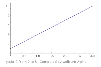
 where m is the slope of the line (
 or
or  ) and b is where the line crosses the y axis.
 (which puts you at
  ), and let’s say that you want to go downhill from where you were at. You could do that by looking at the slope / derivative at that point, which is 3 (it’s 3 for every point on the line). Since the derivative is positive, that means going to the right will make the y value larger (you’ll go up hill) and going to the left will make the y value smaller (you’ll go down hill).
 ?
?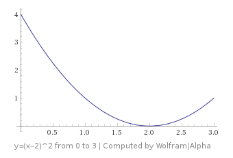
 . Now, which way do you move to go downhill?
 , which you can plug your x value into to get the slope / derivative at that point: -2.
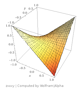
 , and let’s say that we want to go down hill. Instead of just having one variable to take the derivative of (x), we now have two variables (x and y). How are we going to deal with this?
 . That tells us how much we would add to z if we added one to x. It’s a slope that is specifically down the x axis.


 which looks like this:
 which ended up working better for me:
 – and the mantissa tells you where you are in that range.


 ) into “mantissa”. The result tells us the range that we’ll get the precision at.
 .
.
 ).
).
 to
to  .
. )
) )
) )
)