Random numbers can be useful in graphics and game development, but they have a pesky and sometimes undesirable habit of clumping together.
This is a problem in path tracing and monte carlo integration when you take N samples, but the samples aren’t well spread across the sampling range.
This can also be a problem for situations like when you are randomly placing objects in the world or generating treasure for a treasure chest. You don’t want your randomly placed trees to only be in one part of the forest, and you don’t want a player to get only trash items or only godly items when they open a treasure chest. Ideally you want to have some randomness, but you don’t want the random number generator to give you all of the same or similar random numbers.
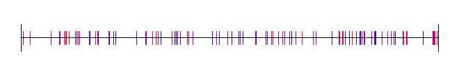
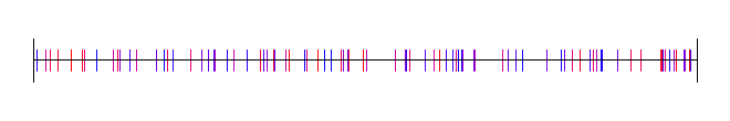
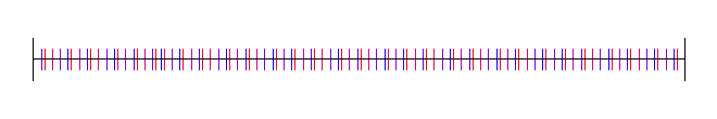
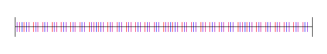
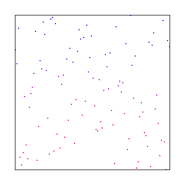
The problem is that random numbers can be TOO random, like in the below where you can see clumps and large gaps between the 100 samples.
For cases like that, when you want random numbers that are a little bit more well distributed, you might find some use in low discrepancy sequences.
The standalone C++ code (one source file, standard headers, no libraries to link to) I used to generate the data and images are at the bottom of this post, as well as some links to more resources.
What Is Discrepancy?
In this context, discrepancy is a measurement of the highest or lowest density of points in a sequence. High discrepancy means that there is either a large area of empty space, or that there is an area that has a high density of points. Low discrepancy means that there are neither, and that your points are more or less pretty evenly distributed.
The lowest discrepancy possible has no randomness at all, and in the 1 dimensional case means that the points are evenly distributed on a grid. For monte carlo integration and the game dev usage cases I mentioned, we do want some randomness, we just want the random points to be spread out a little more evenly.
If more formal math notation is your thing, discrepancy is defined as:
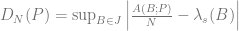
You can read more about the formal definition here: Wikipedia:
Equidistributed sequence
For monte carlo integration specifically, this is the behavior each thing gives you:
- High Discrepancy: Random Numbers / White Noise aka Uniform Distribution – At lower sample counts, convergance is slower (and have higher variance) due to the possibility of not getting good coverage over the area you integrating. At higher sample counts, this problem disappears. (Hint: real time graphics and preview renderings use a smaller number of samples)
- Lowest Discrepancy: Regular Grid – This will cause aliasing, unlike the other “random” based sampling, which trade aliasing for noise. Noise is preferred over aliasing.
- Low Discrepancy: Low Discrepancy Sequences – In lower numbers of samples, this will have faster convergence by having better coverage of the sampling space, but will use randomness to get rid of aliasing by introducing noise.
Also interesting to note, Quasi Monte Carlo has provably better asymptotic convergence than regular monte carlo integration.
1 Dimensional Sequences
We’ll first look at 1 dimensional sequences.
Grid
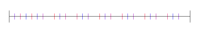
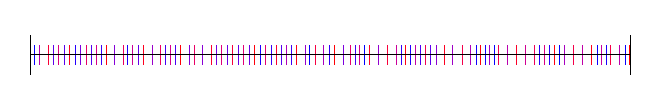
Here are 100 samples evenly spaced:
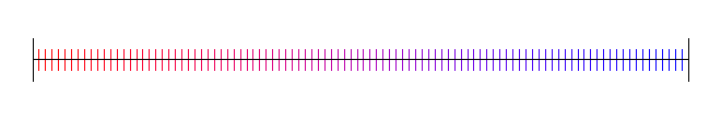
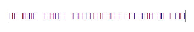
Random Numbers (White Noise)
This is actually a high discrepancy sequence. To generate this, you just use a standard random number generator to pick 100 points between 0 and 1. I used std::mt19937 with a std::uniform_real_distribution from 0 to 1:
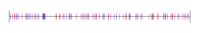
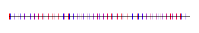
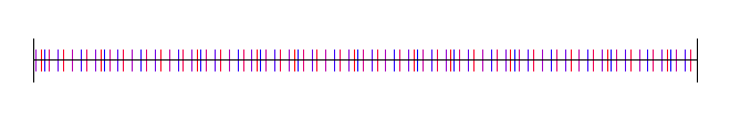
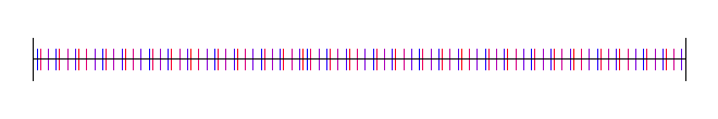
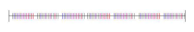
Subrandom Numbers
Subrandom numbers are ways to decrease the discrepancy of white noise.
One way to do this is to break the sampling space in half. You then generate even numbered samples in the first half of the space, and odd numbered samples in the second half of the space.

There’s no reason you can’t generalize this into more divisions of space though.
This splits the space into 4 regions:
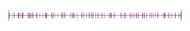
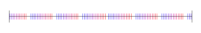
8 regions:

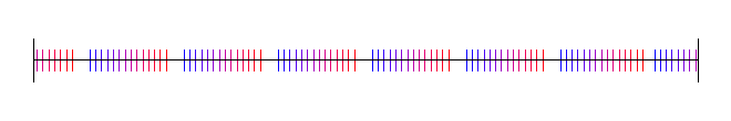
16 regions:
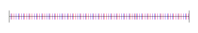
32 regions:
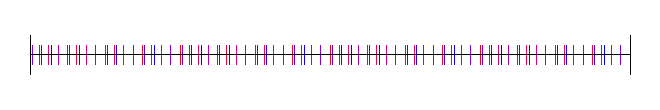
There are other ways to generate subrandom numbers though. One way is to generate random numbers between 0 and 0.5, and add them to the last sample, plus 0.5. This gives you a random walk type setup.
Here is that:
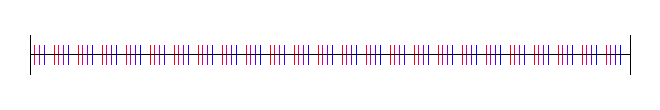
Uniform Sampling + Jitter
If you take the first subrandom idea to the logical maximum, you break your sample space up into N sections and place one point within those N sections to make a low discrepancy sequence made up of N points.
Another way to look at this is that you do uniform sampling, but add some random jitter to the samples, between +/- half a uniform sample size, to keep the samples in their own areas.
This is that:
I have heard that Pixar invented this technique interestingly.
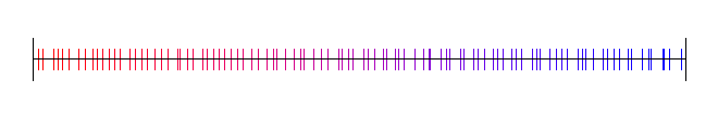
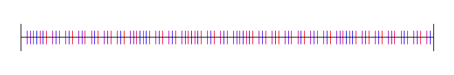
Irrational Numbers
Rational numbers are numbers which can be described as fractions, such as 0.75 which can be expressed as 3/4. Irrational numbers are numbers which CANNOT be described as fractions, such as pi, or the golden ratio, or the square root of a prime number.
Interestingly you can use irrational numbers to generate low discrepancy sequences. You start with some value (could be 0, or could be a random number), add the irrational number, and modulus against 1.0. To get the next sample you add the irrational value again, and modulus against 1.0 again. Rinse and repeat until you get as many samples as you want.
Some values work better than others though, and apparently the golden ratio is provably the best choice (1.61803398875…), says Wikipedia.
Here is the golden ratio, using 4 different random (white noise) starting values:
Here I’ve used the square root of 2, with 4 different starting random numbers again:

Lastly, here is pi, with 4 random starting values:

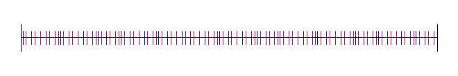
Van der Corput Sequence
The Van der Corput sequence is the 1d equivelant of the Halton sequence which we’ll talk about later.
How you generate values in the Van der Corput sequence is you convert the index of your sample into some base.
For instance if it was base 2, you would convert your index to binary. If it was base 16, you would convert your index to hexadecimal.
Now, instead of treating the digits as if they are 


To show a couple quick examples, let’s say we wanted sample 6 in the sequence of base 2.
First we convert 6 to binary which is 110. From right to left, we have 3 digits: a 0 in the 1’s place, a 1 in the 2’s place, and a 1 in the 4’s place. 
To get the Van der Corput value for this, instead of treating it as the 1’s, 2’s and 4’s digit, we treat it as the 1/2, 1/4 and 1/8’s digit.

So, sample 6 in the Van der Corput sequence using base 2 is 3/8.
Let’s try sample 21 in base 3.
First we convert 21 to base 3 which is 210. We can verify this is right by seeing that 
Instead of a 1’s, 3’s and 9’s digit, we are going to treat it like a 1/3, 1/9 and 1/27 digit.

So, sample 21 in the Van der Corput sequence using base 3 is 5/27.
Here is the Van der Corput sequence for base 2:
Here it is for base 3:

Base 4:
Base 5:
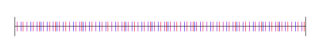
Sobol
One dimensional Sobol is actually just the Van der Corput sequence base 2 re-arranged a little bit, but it’s generated differently.
You start with 0 (either using it as sample 0 or sample -1, doesn’t matter which), and for each sample you do this:
- Calculate the Ruler function value for the current sample’s index(more info in a second)
- Make the direction vector by shifting 1 left (in binary) 31 – ruler times.
- XOR the last sample by the direction vector to get the new sample
- To interpret the sample as a floating point number you divide it by
That might sound completely different than the Van der Corput sequence but it actually is the same thing – just re-ordered.
In the final step when dividing by 
The Ruler Function goes like: 0, 1, 0, 2, 0, 1, 0, 3, 0, 1, 0, 2, 0, 1, 0, …
It’s pretty easy to calculate too. Calculating the ruler function for an index (starting at 1) is just the zero based index of the right most 1’s digit after converting the number to binary.
1 in binary is 001 so Ruler(1) is 0.
2 in binary is 010 so Ruler(2) is 1.
3 in binary is 011 so Ruler(3) is 0.
4 in binary is 100 so Ruler(4) is 2.
5 in binary is 101 so Ruler(5) is 0.
and so on.
Here is 1D Sobol:
Hammersley
In one dimension, the Hammersley sequence is the same as the base 2 Van der Corput sequence, and in the same order. If that sounds strange that it’s the same, it’s a 2d sequence I broke down into a 1d sequence for comparison. The one thing Hammersley has that makes it unique in the 1d case is that you can truncate bits.
It doesn’t seem that useful for 1d Hammersley to truncate bits but knowing that is useful info too I guess. Look at the 2d version of Hammersley to get a fairer look at it, because it’s meant to be a 2d sequence.
Here is Hammersley:

With 1 bit truncated:

With 2 bits truncated:
Poisson Disc
Poisson disc points are points which are densely packed, but have a minimum distance from each other.
Computer scientists are still working out good algorithms to generate these points efficiently.
I use “Mitchell’s Best-Candidate” which means that when you want to generate a new point in the sequence, you generate N new points, and choose whichever point is farthest away from the other points you’ve generated so far.
Here it is where N is 100:
2 Dimensional Sequences
Next up, let’s look at some 2 dimensional sequences.
Grid
Below is 2d uniform samples on a grid.
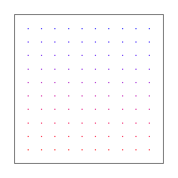
Note that uniform grid is not particularly low discrepancy for the 2d case! More info here: Is it expected that uniform points would have non zero discrepancy?
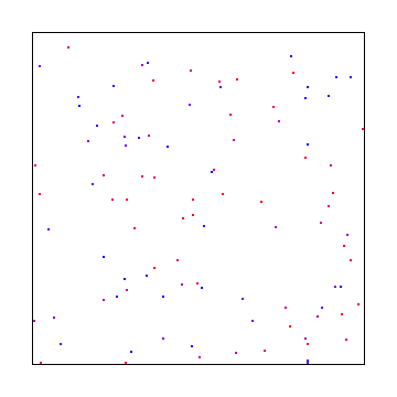
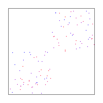
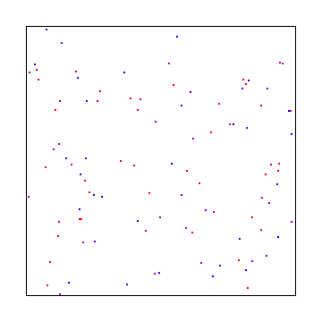
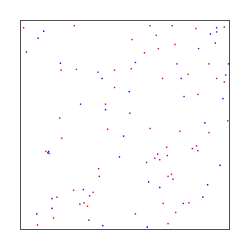
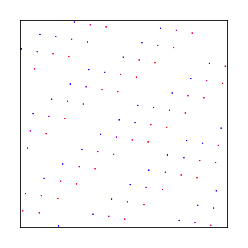
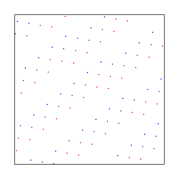
Random
Here are 100 random points:
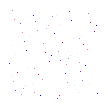
Uniform Grid + Jitter
Here is a uniform grid that has random jitter applied to the points. Jittered grid is a pretty commonly used low discrepancy sampling technique that has good success.

Subrandom
Just like in 1 dimensions, you can apply the subrandom ideas to 2 dimensions where you divide the X and Y axis into so many sections, and randomly choose points in the sections.
If you divide X and Y into the same number of sections though, you are going to have a problem because some areas are not going to have any points in them.
@Reedbeta pointed out that instead of using i%x and i%y, that you could use i%x and (i/x)%y to make it pick points in all regions.
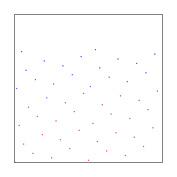
Picking different numbers for X and Y can be another way to give good results. Here’s dividing X and Y into 2 and 3 sections respectively:
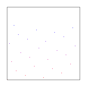
If you choose co-prime numbers for divisions for each axis you can get maximal period of repeats. 2 and 3 are coprime so the last example is a good example of that, but here is 3 and 11:
Here is 3 and 97. 97 is large enough that with only doing 100 samples, we are almost doing jittered grid on the y axis.
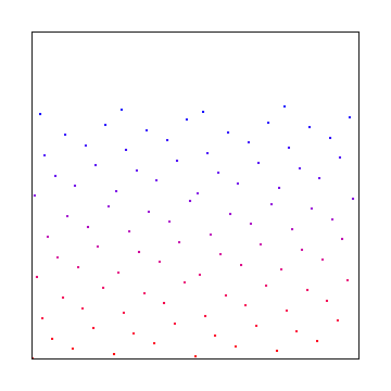
Here is the other subrandom number from 1d, where we start with a random value for X and Y, and then add a random number between 0 and 0.5 to each, also adding 0.5, to make a “random walk” type setup again:
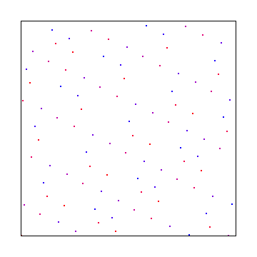
Halton
The Halton sequence is just the Van der Corput sequence, but using a different base on each axis.
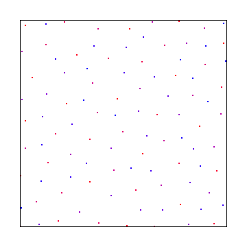
Here is the Halton sequence where X and Y use bases 2 and 3:
Here it is using bases 5 and 7:
Here are bases 13 and 9:
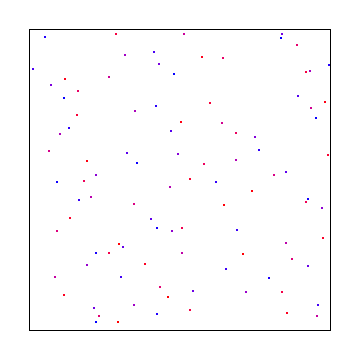
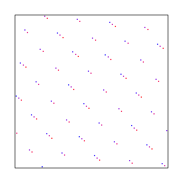
Irrational Numbers
The irrational numbers technique can be used for 2d as well but I wasn’t able to find out how to make it give decent looking output that didn’t have an obvious diagonal pattern in them. Bart Wronski shared a neat paper that explains how to use the golden ratio in 2d with great success: Golden Ratio Sequences For Low-Discrepancy Sampling
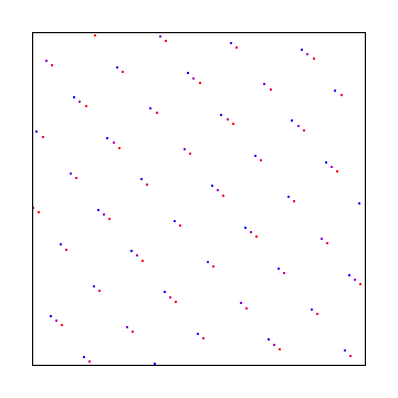
This uses the golden ratio for the X axis and the square root of 2 for the Y axis. Below that is the same, with a random starting point, to make it give a different sequence.
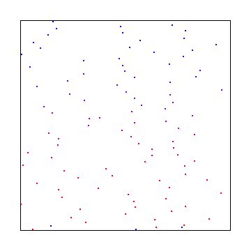
Here X axis uses square root of 2 and Y axis uses square root of 3. Below that is a random starting point, which gives the same discrepancy.
Hammersley
In 2 dimensions, the Hammersley sequence uses the 1d Hammersley sequence for the X axis: Instead of treating the binary version of the index as binary, you treat it as fractions like you do for Van der Corput and sum up the fractions.
For the Y axis, you just reverse the bits and then do the same!
Here is the Hammersley sequence. Note we would have to take 128 samples (not just the 100 we did) if we wanted it to fill the entire square with samples.
Truncating bits in 2d is a bit useful. Here is 1 bit truncated:
2 bits truncated:
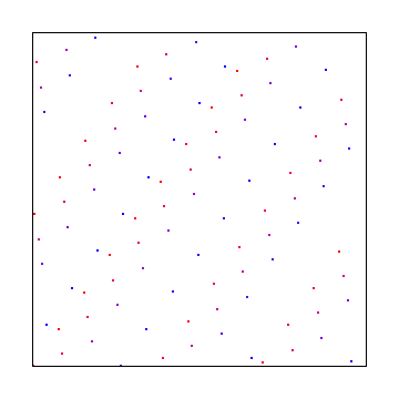
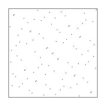
Poisson Disc
Using the same method we did for 1d, we can generate points in 2d space:
N Rooks
There is a sampling pattern called N-Rooks where you put N rooks onto a chess board and arrange them such that no two are in the same row or column.
A way to generate these samples is to realize that there will be only one rook per row, and that none of them will ever be in the same column. So, you make an array that has numbers 0 to N-1, and then shuffle the array. The index into the array is the row, and the value in the array is the column.
Here are 100 rooks:
Sobol
Sobol in two dimensions is more complex to explain so I’ll link you to the source I used: Sobol Sequences Made Simple.
The 1D sobol already covered is used for the X axis, and then something more complex was used for the Y axis:
Links
Bart Wronski has a really great series on a related topic: Dithering in Games
Wikipedia: Low Discrepancy Sequence
Wikipedia: Van der Corput Sequence
Using Fibonacci Sequence To Generate Colors
Deeper info and usage cases for low discrepancy sequences
Low discrepancy sequences are related to blue noise. Where white noise contains all frequencies evenly, blue noise has more high frequencies and fewer low frequencies. Blue noise is essentially the ultimate in low discrepancy, but can be expensive to compute. Here are some pages on blue noise:
The problem with 3D blue noise
Vegetation placement in “The Witness”
Here are some links from @marc_b_reynolds:
Sobol (low-discrepancy) sequence in 1-3D, stratified in 2-4D.
Classic binary-reflected gray code.
Sobol.h
Code
#define _CRT_SECURE_NO_WARNINGS
#include <windows.h> // for bitmap headers and performance counter. Sorry non windows people!
#include <vector>
#include <stdint.h>
#include <random>
#include <array>
#include <algorithm>
#include <stdlib.h>
#include <set>
typedef uint8_t uint8;
#define NUM_SAMPLES 100 // to simplify some 2d code, this must be a square
#define NUM_SAMPLES_FOR_COLORING 100
// Turning this on will slow things down significantly because it's an O(N^5) operation for 2d!
#define CALCULATE_DISCREPANCY 0
#define IMAGE1D_WIDTH 600
#define IMAGE1D_HEIGHT 50
#define IMAGE2D_WIDTH 300
#define IMAGE2D_HEIGHT 300
#define IMAGE_PAD 30
#define IMAGE1D_CENTERX ((IMAGE1D_WIDTH+IMAGE_PAD*2)/2)
#define IMAGE1D_CENTERY ((IMAGE1D_HEIGHT+IMAGE_PAD*2)/2)
#define IMAGE2D_CENTERX ((IMAGE2D_WIDTH+IMAGE_PAD*2)/2)
#define IMAGE2D_CENTERY ((IMAGE2D_HEIGHT+IMAGE_PAD*2)/2)
#define AXIS_HEIGHT 40
#define DATA_HEIGHT 20
#define DATA_WIDTH 2
#define COLOR_FILL SColor(255,255,255)
#define COLOR_AXIS SColor(0, 0, 0)
//======================================================================================
struct SImageData
{
SImageData ()
: m_width(0)
, m_height(0)
{ }
size_t m_width;
size_t m_height;
size_t m_pitch;
std::vector<uint8> m_pixels;
};
struct SColor
{
SColor (uint8 _R = 0, uint8 _G = 0, uint8 _B = 0)
: R(_R), G(_G), B(_B)
{ }
uint8 B, G, R;
};
//======================================================================================
bool SaveImage (const char *fileName, const SImageData &image)
{
// open the file if we can
FILE *file;
file = fopen(fileName, "wb");
if (!file) {
printf("Could not save %s\n", fileName);
return false;
}
// make the header info
BITMAPFILEHEADER header;
BITMAPINFOHEADER infoHeader;
header.bfType = 0x4D42;
header.bfReserved1 = 0;
header.bfReserved2 = 0;
header.bfOffBits = 54;
infoHeader.biSize = 40;
infoHeader.biWidth = (LONG)image.m_width;
infoHeader.biHeight = (LONG)image.m_height;
infoHeader.biPlanes = 1;
infoHeader.biBitCount = 24;
infoHeader.biCompression = 0;
infoHeader.biSizeImage = (DWORD) image.m_pixels.size();
infoHeader.biXPelsPerMeter = 0;
infoHeader.biYPelsPerMeter = 0;
infoHeader.biClrUsed = 0;
infoHeader.biClrImportant = 0;
header.bfSize = infoHeader.biSizeImage + header.bfOffBits;
// write the data and close the file
fwrite(&header, sizeof(header), 1, file);
fwrite(&infoHeader, sizeof(infoHeader), 1, file);
fwrite(&image.m_pixels[0], infoHeader.biSizeImage, 1, file);
fclose(file);
return true;
}
//======================================================================================
void ImageInit (SImageData& image, size_t width, size_t height)
{
image.m_width = width;
image.m_height = height;
image.m_pitch = 4 * ((width * 24 + 31) / 32);
image.m_pixels.resize(image.m_pitch * image.m_width);
std::fill(image.m_pixels.begin(), image.m_pixels.end(), 0);
}
//======================================================================================
void ImageClear (SImageData& image, const SColor& color)
{
uint8* row = &image.m_pixels[0];
for (size_t rowIndex = 0; rowIndex < image.m_height; ++rowIndex)
{
SColor* pixels = (SColor*)row;
std::fill(pixels, pixels + image.m_width, color);
row += image.m_pitch;
}
}
//======================================================================================
void ImageBox (SImageData& image, size_t x1, size_t x2, size_t y1, size_t y2, const SColor& color)
{
for (size_t y = y1; y < y2; ++y)
{
uint8* row = &image.m_pixels[y * image.m_pitch];
SColor* start = &((SColor*)row)[x1];
std::fill(start, start + x2 - x1, color);
}
}
//======================================================================================
float Distance (float x1, float y1, float x2, float y2)
{
float dx = (x2 - x1);
float dy = (y2 - y1);
return std::sqrtf(dx*dx + dy*dy);
}
//======================================================================================
SColor DataPointColor (size_t sampleIndex)
{
SColor ret;
float percent = (float(sampleIndex) / (float(NUM_SAMPLES_FOR_COLORING) - 1.0f));
ret.R = uint8((1.0f - percent) * 255.0f);
ret.G = 0;
ret.B = uint8(percent * 255.0f);
float mag = (float)sqrt(ret.R*ret.R + ret.G*ret.G + ret.B*ret.B);
ret.R = uint8((float(ret.R) / mag)*255.0f);
ret.G = uint8((float(ret.G) / mag)*255.0f);
ret.B = uint8((float(ret.B) / mag)*255.0f);
return ret;
}
//======================================================================================
float RandomFloat (float min, float max)
{
static std::random_device rd;
static std::mt19937 mt(rd());
std::uniform_real_distribution<float> dist(min, max);
return dist(mt);
}
//======================================================================================
size_t Ruler (size_t n)
{
size_t ret = 0;
while (n != 0 && (n & 1) == 0)
{
n /= 2;
++ret;
}
return ret;
}
//======================================================================================
float CalculateDiscrepancy1D (const std::array<float, NUM_SAMPLES>& samples)
{
// some info about calculating discrepancy
// https://math.stackexchange.com/questions/1681562/how-to-calculate-discrepancy-of-a-sequence
// Calculates the discrepancy of this data.
// Assumes the data is [0,1) for valid sample range
std::array<float, NUM_SAMPLES> sortedSamples = samples;
std::sort(sortedSamples.begin(), sortedSamples.end());
float maxDifference = 0.0f;
for (size_t startIndex = 0; startIndex <= NUM_SAMPLES; ++startIndex)
{
// startIndex 0 = 0.0f. startIndex 1 = sortedSamples[0]. etc
float startValue = 0.0f;
if (startIndex > 0)
startValue = sortedSamples[startIndex - 1];
for (size_t stopIndex = startIndex; stopIndex <= NUM_SAMPLES; ++stopIndex)
{
// stopIndex 0 = sortedSamples[0]. startIndex[N] = 1.0f. etc
float stopValue = 1.0f;
if (stopIndex < NUM_SAMPLES)
stopValue = sortedSamples[stopIndex];
float length = stopValue - startValue;
// open interval (startValue, stopValue)
size_t countInside = 0;
for (float sample : samples)
{
if (sample > startValue &&
sample < stopValue)
{
++countInside;
}
}
float density = float(countInside) / float(NUM_SAMPLES);
float difference = std::abs(density - length);
if (difference > maxDifference)
maxDifference = difference;
// closed interval [startValue, stopValue]
countInside = 0;
for (float sample : samples)
{
if (sample >= startValue &&
sample <= stopValue)
{
++countInside;
}
}
density = float(countInside) / float(NUM_SAMPLES);
difference = std::abs(density - length);
if (difference > maxDifference)
maxDifference = difference;
}
}
return maxDifference;
}
//======================================================================================
float CalculateDiscrepancy2D (const std::array<std::array<float, 2>, NUM_SAMPLES>& samples)
{
// some info about calculating discrepancy
// https://math.stackexchange.com/questions/1681562/how-to-calculate-discrepancy-of-a-sequence
// Calculates the discrepancy of this data.
// Assumes the data is [0,1) for valid sample range.
// Get the sorted list of unique values on each axis
std::set<float> setSamplesX;
std::set<float> setSamplesY;
for (const std::array<float, 2>& sample : samples)
{
setSamplesX.insert(sample[0]);
setSamplesY.insert(sample[1]);
}
std::vector<float> sortedXSamples;
std::vector<float> sortedYSamples;
sortedXSamples.reserve(setSamplesX.size());
sortedYSamples.reserve(setSamplesY.size());
for (float f : setSamplesX)
sortedXSamples.push_back(f);
for (float f : setSamplesY)
sortedYSamples.push_back(f);
// Get the sorted list of samples on the X axis, for faster interval testing
std::array<std::array<float, 2>, NUM_SAMPLES> sortedSamplesX = samples;
std::sort(sortedSamplesX.begin(), sortedSamplesX.end(),
[] (const std::array<float, 2>& itemA, const std::array<float, 2>& itemB)
{
return itemA[0] < itemB[0];
}
);
// calculate discrepancy
float maxDifference = 0.0f;
for (size_t startIndexY = 0; startIndexY <= sortedYSamples.size(); ++startIndexY)
{
float startValueY = 0.0f;
if (startIndexY > 0)
startValueY = *(sortedYSamples.begin() + startIndexY - 1);
for (size_t startIndexX = 0; startIndexX <= sortedXSamples.size(); ++startIndexX)
{
float startValueX = 0.0f;
if (startIndexX > 0)
startValueX = *(sortedXSamples.begin() + startIndexX - 1);
for (size_t stopIndexY = startIndexY; stopIndexY <= sortedYSamples.size(); ++stopIndexY)
{
float stopValueY = 1.0f;
if (stopIndexY < sortedYSamples.size())
stopValueY = sortedYSamples[stopIndexY];
for (size_t stopIndexX = startIndexX; stopIndexX <= sortedXSamples.size(); ++stopIndexX)
{
float stopValueX = 1.0f;
if (stopIndexX < sortedXSamples.size())
stopValueX = sortedXSamples[stopIndexX];
// calculate area
float length = stopValueX - startValueX;
float height = stopValueY - startValueY;
float area = length * height;
// open interval (startValue, stopValue)
size_t countInside = 0;
for (const std::array<float, 2>& sample : samples)
{
if (sample[0] > startValueX &&
sample[1] > startValueY &&
sample[0] < stopValueX &&
sample[1] < stopValueY)
{
++countInside;
}
}
float density = float(countInside) / float(NUM_SAMPLES);
float difference = std::abs(density - area);
if (difference > maxDifference)
maxDifference = difference;
// closed interval [startValue, stopValue]
countInside = 0;
for (const std::array<float, 2>& sample : samples)
{
if (sample[0] >= startValueX &&
sample[1] >= startValueY &&
sample[0] <= stopValueX &&
sample[1] <= stopValueY)
{
++countInside;
}
}
density = float(countInside) / float(NUM_SAMPLES);
difference = std::abs(density - area);
if (difference > maxDifference)
maxDifference = difference;
}
}
}
}
return maxDifference;
}
//======================================================================================
void Test1D (const char* fileName, const std::array<float, NUM_SAMPLES>& samples)
{
// create and clear the image
SImageData image;
ImageInit(image, IMAGE1D_WIDTH + IMAGE_PAD * 2, IMAGE1D_HEIGHT + IMAGE_PAD * 2);
// setup the canvas
ImageClear(image, COLOR_FILL);
// calculate the discrepancy
#if CALCULATE_DISCREPANCY
float discrepancy = CalculateDiscrepancy1D(samples);
printf("%s Discrepancy = %0.2f%%\n", fileName, discrepancy*100.0f);
#endif
// draw the sample points
size_t i = 0;
for (float f: samples)
{
size_t pos = size_t(f * float(IMAGE1D_WIDTH)) + IMAGE_PAD;
ImageBox(image, pos, pos + 1, IMAGE1D_CENTERY - DATA_HEIGHT / 2, IMAGE1D_CENTERY + DATA_HEIGHT / 2, DataPointColor(i));
++i;
}
// draw the axes lines. horizontal first then the two vertical
ImageBox(image, IMAGE_PAD, IMAGE1D_WIDTH + IMAGE_PAD, IMAGE1D_CENTERY, IMAGE1D_CENTERY + 1, COLOR_AXIS);
ImageBox(image, IMAGE_PAD, IMAGE_PAD + 1, IMAGE1D_CENTERY - AXIS_HEIGHT / 2, IMAGE1D_CENTERY + AXIS_HEIGHT / 2, COLOR_AXIS);
ImageBox(image, IMAGE1D_WIDTH + IMAGE_PAD, IMAGE1D_WIDTH + IMAGE_PAD + 1, IMAGE1D_CENTERY - AXIS_HEIGHT / 2, IMAGE1D_CENTERY + AXIS_HEIGHT / 2, COLOR_AXIS);
// save the image
SaveImage(fileName, image);
}
//======================================================================================
void Test2D (const char* fileName, const std::array<std::array<float,2>, NUM_SAMPLES>& samples)
{
// create and clear the image
SImageData image;
ImageInit(image, IMAGE2D_WIDTH + IMAGE_PAD * 2, IMAGE2D_HEIGHT + IMAGE_PAD * 2);
// setup the canvas
ImageClear(image, COLOR_FILL);
// calculate the discrepancy
#if CALCULATE_DISCREPANCY
float discrepancy = CalculateDiscrepancy2D(samples);
printf("%s Discrepancy = %0.2f%%\n", fileName, discrepancy*100.0f);
#endif
// draw the sample points
size_t i = 0;
for (const std::array<float, 2>& sample : samples)
{
size_t posx = size_t(sample[0] * float(IMAGE2D_WIDTH)) + IMAGE_PAD;
size_t posy = size_t(sample[1] * float(IMAGE2D_WIDTH)) + IMAGE_PAD;
ImageBox(image, posx - 1, posx + 1, posy - 1, posy + 1, DataPointColor(i));
++i;
}
// horizontal lines
ImageBox(image, IMAGE_PAD - 1, IMAGE2D_WIDTH + IMAGE_PAD + 1, IMAGE_PAD - 1, IMAGE_PAD, COLOR_AXIS);
ImageBox(image, IMAGE_PAD - 1, IMAGE2D_WIDTH + IMAGE_PAD + 1, IMAGE2D_HEIGHT + IMAGE_PAD, IMAGE2D_HEIGHT + IMAGE_PAD + 1, COLOR_AXIS);
// vertical lines
ImageBox(image, IMAGE_PAD - 1, IMAGE_PAD, IMAGE_PAD - 1, IMAGE2D_HEIGHT + IMAGE_PAD + 1, COLOR_AXIS);
ImageBox(image, IMAGE_PAD + IMAGE2D_WIDTH, IMAGE_PAD + IMAGE2D_WIDTH + 1, IMAGE_PAD - 1, IMAGE2D_HEIGHT + IMAGE_PAD + 1, COLOR_AXIS);
// save the image
SaveImage(fileName, image);
}
//======================================================================================
void TestUniform1D (bool jitter)
{
// calculate the sample points
const float c_cellSize = 1.0f / float(NUM_SAMPLES+1);
std::array<float, NUM_SAMPLES> samples;
for (size_t i = 0; i < NUM_SAMPLES; ++i)
{
samples[i] = float(i+1) / float(NUM_SAMPLES+1);
if (jitter)
samples[i] += RandomFloat(-c_cellSize*0.5f, c_cellSize*0.5f);
}
// save bitmap etc
if (jitter)
Test1D("1DUniformJitter.bmp", samples);
else
Test1D("1DUniform.bmp", samples);
}
//======================================================================================
void TestUniformRandom1D ()
{
// calculate the sample points
const float c_halfJitter = 1.0f / float((NUM_SAMPLES + 1) * 2);
std::array<float, NUM_SAMPLES> samples;
for (size_t i = 0; i < NUM_SAMPLES; ++i)
samples[i] = RandomFloat(0.0f, 1.0f);
// save bitmap etc
Test1D("1DUniformRandom.bmp", samples);
}
//======================================================================================
void TestSubRandomA1D (size_t numRegions)
{
const float c_randomRange = 1.0f / float(numRegions);
// calculate the sample points
const float c_halfJitter = 1.0f / float((NUM_SAMPLES + 1) * 2);
std::array<float, NUM_SAMPLES> samples;
for (size_t i = 0; i < NUM_SAMPLES; ++i)
{
samples[i] = RandomFloat(0.0f, c_randomRange);
samples[i] += float(i % numRegions) / float(numRegions);
}
// save bitmap etc
char fileName[256];
sprintf(fileName, "1DSubRandomA_%zu.bmp", numRegions);
Test1D(fileName, samples);
}
//======================================================================================
void TestSubRandomB1D ()
{
// calculate the sample points
std::array<float, NUM_SAMPLES> samples;
float sample = RandomFloat(0.0f, 0.5f);
for (size_t i = 0; i < NUM_SAMPLES; ++i)
{
sample = std::fmodf(sample + 0.5f + RandomFloat(0.0f, 0.5f), 1.0f);
samples[i] = sample;
}
// save bitmap etc
Test1D("1DSubRandomB.bmp", samples);
}
//======================================================================================
void TestVanDerCorput (size_t base)
{
// calculate the sample points
std::array<float, NUM_SAMPLES> samples;
for (size_t i = 0; i < NUM_SAMPLES; ++i)
{
samples[i] = 0.0f;
float denominator = float(base);
size_t n = i;
while (n > 0)
{
size_t multiplier = n % base;
samples[i] += float(multiplier) / denominator;
n = n / base;
denominator *= base;
}
}
// save bitmap etc
char fileName[256];
sprintf(fileName, "1DVanDerCorput_%zu.bmp", base);
Test1D(fileName, samples);
}
//======================================================================================
void TestIrrational1D (float irrational, float seed)
{
// calculate the sample points
std::array<float, NUM_SAMPLES> samples;
float sample = seed;
for (size_t i = 0; i < NUM_SAMPLES; ++i)
{
sample = std::fmodf(sample + irrational, 1.0f);
samples[i] = sample;
}
// save bitmap etc
char irrationalStr[256];
sprintf(irrationalStr, "%f", irrational);
char seedStr[256];
sprintf(seedStr, "%f", seed);
char fileName[256];
sprintf(fileName, "1DIrrational_%s_%s.bmp", &irrationalStr[2], &seedStr[2]);
Test1D(fileName, samples);
}
//======================================================================================
void TestSobol1D ()
{
// calculate the sample points
std::array<float, NUM_SAMPLES> samples;
size_t sampleInt = 0;
for (size_t i = 0; i < NUM_SAMPLES; ++i)
{
size_t ruler = Ruler(i + 1);
size_t direction = size_t(size_t(1) << size_t(31 - ruler));
sampleInt = sampleInt ^ direction;
samples[i] = float(sampleInt) / std::pow(2.0f, 32.0f);
}
// save bitmap etc
Test1D("1DSobol.bmp", samples);
}
//======================================================================================
void TestHammersley1D (size_t truncateBits)
{
// calculate the sample points
std::array<float, NUM_SAMPLES> samples;
size_t sampleInt = 0;
for (size_t i = 0; i < NUM_SAMPLES; ++i)
{
size_t n = i >> truncateBits;
float base = 1.0f / 2.0f;
samples[i] = 0.0f;
while (n)
{
if (n & 1)
samples[i] += base;
n /= 2;
base /= 2.0f;
}
}
// save bitmap etc
char fileName[256];
sprintf(fileName, "1DHammersley_%zu.bmp", truncateBits);
Test1D(fileName, samples);
}
//======================================================================================
float MinimumDistance1D (const std::array<float, NUM_SAMPLES>& samples, size_t numSamples, float x)
{
// Used by poisson.
// This returns the minimum distance that point (x) is away from the sample points, from [0, numSamples).
float minimumDistance = 0.0f;
for (size_t i = 0; i < numSamples; ++i)
{
float distance = std::abs(samples[i] - x);
if (i == 0 || distance < minimumDistance)
minimumDistance = distance;
}
return minimumDistance;
}
//======================================================================================
void TestPoisson1D ()
{
// every time we want to place a point, we generate this many points and choose the one farthest away from all the other points (largest minimum distance)
const size_t c_bestOfAttempts = 100;
// calculate the sample points
std::array<float, NUM_SAMPLES> samples;
for (size_t sampleIndex = 0; sampleIndex < NUM_SAMPLES; ++sampleIndex)
{
// generate some random points and keep the one that has the largest minimum distance from any of the existing points
float bestX = 0.0f;
float bestMinDistance = 0.0f;
for (size_t attempt = 0; attempt < c_bestOfAttempts; ++attempt)
{
float attemptX = RandomFloat(0.0f, 1.0f);
float minDistance = MinimumDistance1D(samples, sampleIndex, attemptX);
if (minDistance > bestMinDistance)
{
bestX = attemptX;
bestMinDistance = minDistance;
}
}
samples[sampleIndex] = bestX;
}
// save bitmap etc
Test1D("1DPoisson.bmp", samples);
}
//======================================================================================
void TestUniform2D (bool jitter)
{
// calculate the sample points
std::array<std::array<float, 2>, NUM_SAMPLES> samples;
const size_t c_oneSide = size_t(std::sqrt(NUM_SAMPLES));
const float c_cellSize = 1.0f / float(c_oneSide+1);
for (size_t iy = 0; iy < c_oneSide; ++iy)
{
for (size_t ix = 0; ix < c_oneSide; ++ix)
{
size_t sampleIndex = iy * c_oneSide + ix;
samples[sampleIndex][0] = float(ix + 1) / (float(c_oneSide + 1));
if (jitter)
samples[sampleIndex][0] += RandomFloat(-c_cellSize*0.5f, c_cellSize*0.5f);
samples[sampleIndex][1] = float(iy + 1) / (float(c_oneSide) + 1.0f);
if (jitter)
samples[sampleIndex][1] += RandomFloat(-c_cellSize*0.5f, c_cellSize*0.5f);
}
}
// save bitmap etc
if (jitter)
Test2D("2DUniformJitter.bmp", samples);
else
Test2D("2DUniform.bmp", samples);
}
//======================================================================================
void TestUniformRandom2D ()
{
// calculate the sample points
std::array<std::array<float, 2>, NUM_SAMPLES> samples;
const size_t c_oneSide = size_t(std::sqrt(NUM_SAMPLES));
const float c_halfJitter = 1.0f / float((c_oneSide + 1) * 2);
for (size_t i = 0; i < NUM_SAMPLES; ++i)
{
samples[i][0] = RandomFloat(0.0f, 1.0f);
samples[i][1] = RandomFloat(0.0f, 1.0f);
}
// save bitmap etc
Test2D("2DUniformRandom.bmp", samples);
}
//======================================================================================
void TestSubRandomA2D (size_t regionsX, size_t regionsY)
{
const float c_randomRangeX = 1.0f / float(regionsX);
const float c_randomRangeY = 1.0f / float(regionsY);
// calculate the sample points
std::array<std::array<float, 2>, NUM_SAMPLES> samples;
for (size_t i = 0; i < NUM_SAMPLES; ++i)
{
samples[i][0] = RandomFloat(0.0f, c_randomRangeX);
samples[i][0] += float(i % regionsX) / float(regionsX);
samples[i][1] = RandomFloat(0.0f, c_randomRangeY);
samples[i][1] += float(i % regionsY) / float(regionsY);
}
// save bitmap etc
char fileName[256];
sprintf(fileName, "2DSubRandomA_%zu_%zu.bmp", regionsX, regionsY);
Test2D(fileName, samples);
}
//======================================================================================
void TestSubRandomB2D ()
{
// calculate the sample points
float samplex = RandomFloat(0.0f, 0.5f);
float sampley = RandomFloat(0.0f, 0.5f);
std::array<std::array<float, 2>, NUM_SAMPLES> samples;
for (size_t i = 0; i < NUM_SAMPLES; ++i)
{
samplex = std::fmodf(samplex + 0.5f + RandomFloat(0.0f, 0.5f), 1.0f);
sampley = std::fmodf(sampley + 0.5f + RandomFloat(0.0f, 0.5f), 1.0f);
samples[i][0] = samplex;
samples[i][1] = sampley;
}
// save bitmap etc
Test2D("2DSubRandomB.bmp", samples);
}
//======================================================================================
void TestHalton (size_t basex, size_t basey)
{
// calculate the sample points
std::array<std::array<float, 2>, NUM_SAMPLES> samples;
const size_t c_oneSide = size_t(std::sqrt(NUM_SAMPLES));
const float c_halfJitter = 1.0f / float((c_oneSide + 1) * 2);
for (size_t i = 0; i < NUM_SAMPLES; ++i)
{
// x axis
samples[i][0] = 0.0f;
{
float denominator = float(basex);
size_t n = i;
while (n > 0)
{
size_t multiplier = n % basex;
samples[i][0] += float(multiplier) / denominator;
n = n / basex;
denominator *= basex;
}
}
// y axis
samples[i][1] = 0.0f;
{
float denominator = float(basey);
size_t n = i;
while (n > 0)
{
size_t multiplier = n % basey;
samples[i][1] += float(multiplier) / denominator;
n = n / basey;
denominator *= basey;
}
}
}
// save bitmap etc
char fileName[256];
sprintf(fileName, "2DHalton_%zu_%zu.bmp", basex, basey);
Test2D(fileName, samples);
}
//======================================================================================
void TestSobol2D ()
{
// calculate the sample points
// x axis
std::array<std::array<float, 2>, NUM_SAMPLES> samples;
size_t sampleInt = 0;
for (size_t i = 0; i < NUM_SAMPLES; ++i)
{
size_t ruler = Ruler(i + 1);
size_t direction = size_t(size_t(1) << size_t(31 - ruler));
sampleInt = sampleInt ^ direction;
samples[i][0] = float(sampleInt) / std::pow(2.0f, 32.0f);
}
// y axis
// Code adapted from http://web.maths.unsw.edu.au/~fkuo/sobol/
// uses numbers: new-joe-kuo-6.21201
// Direction numbers
std::vector<size_t> V;
V.resize((size_t)ceil(log((double)NUM_SAMPLES) / log(2.0)));
V[0] = size_t(1) << size_t(31);
for (size_t i = 1; i < V.size(); ++i)
V[i] = V[i - 1] ^ (V[i - 1] >> 1);
// Samples
sampleInt = 0;
for (size_t i = 0; i < NUM_SAMPLES; ++i) {
size_t ruler = Ruler(i + 1);
sampleInt = sampleInt ^ V[ruler];
samples[i][1] = float(sampleInt) / std::pow(2.0f, 32.0f);
}
// save bitmap etc
Test2D("2DSobol.bmp", samples);
}
//======================================================================================
void TestHammersley2D (size_t truncateBits)
{
// figure out how many bits we are working in.
size_t value = 1;
size_t numBits = 0;
while (value < NUM_SAMPLES)
{
value *= 2;
++numBits;
}
// calculate the sample points
std::array<std::array<float, 2>, NUM_SAMPLES> samples;
size_t sampleInt = 0;
for (size_t i = 0; i < NUM_SAMPLES; ++i)
{
// x axis
samples[i][0] = 0.0f;
{
size_t n = i >> truncateBits;
float base = 1.0f / 2.0f;
while (n)
{
if (n & 1)
samples[i][0] += base;
n /= 2;
base /= 2.0f;
}
}
// y axis
samples[i][1] = 0.0f;
{
size_t n = i >> truncateBits;
size_t mask = size_t(1) << (numBits - 1 - truncateBits);
float base = 1.0f / 2.0f;
while (mask)
{
if (n & mask)
samples[i][1] += base;
mask /= 2;
base /= 2.0f;
}
}
}
// save bitmap etc
char fileName[256];
sprintf(fileName, "2DHammersley_%zu.bmp", truncateBits);
Test2D(fileName, samples);
}
//======================================================================================
void TestRooks2D ()
{
// make and shuffle rook positions
std::random_device rd;
std::mt19937 mt(rd());
std::array<size_t, NUM_SAMPLES> rookPositions;
for (size_t i = 0; i < NUM_SAMPLES; ++i)
rookPositions[i] = i;
std::shuffle(rookPositions.begin(), rookPositions.end(), mt);
// calculate the sample points
std::array<std::array<float, 2>, NUM_SAMPLES> samples;
for (size_t i = 0; i < NUM_SAMPLES; ++i)
{
// x axis
samples[i][0] = float(rookPositions[i]) / float(NUM_SAMPLES-1);
// y axis
samples[i][1] = float(i) / float(NUM_SAMPLES - 1);
}
// save bitmap etc
Test2D("2DRooks.bmp", samples);
}
//======================================================================================
void TestIrrational2D (float irrationalx, float irrationaly, float seedx, float seedy)
{
// calculate the sample points
std::array<std::array<float, 2>, NUM_SAMPLES> samples;
float samplex = seedx;
float sampley = seedy;
for (size_t i = 0; i < NUM_SAMPLES; ++i)
{
samplex = std::fmodf(samplex + irrationalx, 1.0f);
sampley = std::fmodf(sampley + irrationaly, 1.0f);
samples[i][0] = samplex;
samples[i][1] = sampley;
}
// save bitmap etc
char irrationalxStr[256];
sprintf(irrationalxStr, "%f", irrationalx);
char irrationalyStr[256];
sprintf(irrationalyStr, "%f", irrationaly);
char seedxStr[256];
sprintf(seedxStr, "%f", seedx);
char seedyStr[256];
sprintf(seedyStr, "%f", seedy);
char fileName[256];
sprintf(fileName, "2DIrrational_%s_%s_%s_%s.bmp", &irrationalxStr[2], &irrationalyStr[2], &seedxStr[2], &seedyStr[2]);
Test2D(fileName, samples);
}
//======================================================================================
float MinimumDistance2D (const std::array<std::array<float, 2>, NUM_SAMPLES>& samples, size_t numSamples, float x, float y)
{
// Used by poisson.
// This returns the minimum distance that point (x,y) is away from the sample points, from [0, numSamples).
float minimumDistance = 0.0f;
for (size_t i = 0; i < numSamples; ++i)
{
float distance = Distance(samples[i][0], samples[i][1], x, y);
if (i == 0 || distance < minimumDistance)
minimumDistance = distance;
}
return minimumDistance;
}
//======================================================================================
void TestPoisson2D ()
{
// every time we want to place a point, we generate this many points and choose the one farthest away from all the other points (largest minimum distance)
const size_t c_bestOfAttempts = 100;
// calculate the sample points
std::array<std::array<float, 2>, NUM_SAMPLES> samples;
for (size_t sampleIndex = 0; sampleIndex < NUM_SAMPLES; ++sampleIndex)
{
// generate some random points and keep the one that has the largest minimum distance from any of the existing points
float bestX = 0.0f;
float bestY = 0.0f;
float bestMinDistance = 0.0f;
for (size_t attempt = 0; attempt < c_bestOfAttempts; ++attempt)
{
float attemptX = RandomFloat(0.0f, 1.0f);
float attemptY = RandomFloat(0.0f, 1.0f);
float minDistance = MinimumDistance2D(samples, sampleIndex, attemptX, attemptY);
if (minDistance > bestMinDistance)
{
bestX = attemptX;
bestY = attemptY;
bestMinDistance = minDistance;
}
}
samples[sampleIndex][0] = bestX;
samples[sampleIndex][1] = bestY;
}
// save bitmap etc
Test2D("2DPoisson.bmp", samples);
}
//======================================================================================
int main (int argc, char **argv)
{
// 1D tests
{
TestUniform1D(false);
TestUniform1D(true);
TestUniformRandom1D();
TestSubRandomA1D(2);
TestSubRandomA1D(4);
TestSubRandomA1D(8);
TestSubRandomA1D(16);
TestSubRandomA1D(32);
TestSubRandomB1D();
TestVanDerCorput(2);
TestVanDerCorput(3);
TestVanDerCorput(4);
TestVanDerCorput(5);
// golden ratio mod 1 aka (sqrt(5) - 1)/2
TestIrrational1D(0.618034f, 0.0f);
TestIrrational1D(0.618034f, 0.385180f);
TestIrrational1D(0.618034f, 0.775719f);
TestIrrational1D(0.618034f, 0.287194f);
// sqrt(2) - 1
TestIrrational1D(0.414214f, 0.0f);
TestIrrational1D(0.414214f, 0.385180f);
TestIrrational1D(0.414214f, 0.775719f);
TestIrrational1D(0.414214f, 0.287194f);
// PI mod 1
TestIrrational1D(0.141593f, 0.0f);
TestIrrational1D(0.141593f, 0.385180f);
TestIrrational1D(0.141593f, 0.775719f);
TestIrrational1D(0.141593f, 0.287194f);
TestSobol1D();
TestHammersley1D(0);
TestHammersley1D(1);
TestHammersley1D(2);
TestPoisson1D();
}
// 2D tests
{
TestUniform2D(false);
TestUniform2D(true);
TestUniformRandom2D();
TestSubRandomA2D(2, 2);
TestSubRandomA2D(2, 3);
TestSubRandomA2D(3, 11);
TestSubRandomA2D(3, 97);
TestSubRandomB2D();
TestHalton(2, 3);
TestHalton(5, 7);
TestHalton(13, 9);
TestSobol2D();
TestHammersley2D(0);
TestHammersley2D(1);
TestHammersley2D(2);
TestRooks2D();
// X axis = golden ratio mod 1 aka (sqrt(5)-1)/2
// Y axis = sqrt(2) mod 1
TestIrrational2D(0.618034f, 0.414214f, 0.0f, 0.0f);
TestIrrational2D(0.618034f, 0.414214f, 0.775719f, 0.264045f);
// X axis = sqrt(2) mod 1
// Y axis = sqrt(3) mod 1
TestIrrational2D(std::fmodf((float)std::sqrt(2.0f), 1.0f), std::fmodf((float)std::sqrt(3.0f), 1.0f), 0.0f, 0.0f);
TestIrrational2D(std::fmodf((float)std::sqrt(2.0f), 1.0f), std::fmodf((float)std::sqrt(3.0f), 1.0f), 0.775719f, 0.264045f);
TestPoisson2D();
}
#if CALCULATE_DISCREPANCY
printf("\n");
system("pause");
#endif
}


![\left[\begin{array}{rrrr|rrr} P_{00} & P_{01} & P_{10} & P_{11} & C_0 & C_1 & C_2 \\ 1 & 0 & 0 & 0 & 1 & 0 & 0 \\ 0 & 1 & 1 & 0 & 0 & 2 & 0\\ 0 & 0 & 0 & 1 & 0 & 0 & 1 \end{array}\right]](https://s0.wp.com/latex.php?latex=%5Cleft%5B%5Cbegin%7Barray%7D%7Brrrr%7Crrr%7D+P_%7B00%7D+%26+P_%7B01%7D+%26+P_%7B10%7D+%26+P_%7B11%7D+%26+C_0+%26+C_1+%26+C_2+%5C%5C+1+%26+0+%26+0+%26+0+%26+1+%26+0+%26+0+%5C%5C+0+%26+1+%26+1+%26+0+%26+0+%26+2+%26+0%5C%5C+0+%26+0+%26+0+%26+1+%26+0+%26+0+%26+1+%5Cend%7Barray%7D%5Cright%5D+&bg=ffffff&fg=666666&s=0&c=20201002)
![\left[\begin{array}{rrrrrr|rrrrrr} P_{00} & P_{01} & P_{10} & P_{11} & P_{20} & P_{21} & C_0 & C_1 & C_2 & C_3 & C_4 & C_5\\ 1 & 0 & 0 & 0 & 0 & 0 & 1 & 0 & 0 & 0 & 0 & 0\\ 0 & 1 & 1 & 0 & 0 & 0 & 0 & 2 & 0 & 0 & 0 & 0 \\ 0 & 0 & 0 & 1 & 0 & 0 & 0 & 0 & 1 & 0 & 0 & 0 \\ 0 & 0 & 1 & 0 & 0 & 0 & 0 & 0 & 0 & 1 & 0 & 0 \\ 0 & 0 & 0 & 1 & 1 & 0 & 0 & 0 & 0 & 0 & 2 & 0 \\ 0 & 0 & 0 & 0 & 0 & 1 & 0 & 0 & 0 & 0 & 0 & 1 \end{array}\right]](https://s0.wp.com/latex.php?latex=%5Cleft%5B%5Cbegin%7Barray%7D%7Brrrrrr%7Crrrrrr%7D+P_%7B00%7D+%26+P_%7B01%7D+%26+P_%7B10%7D+%26+P_%7B11%7D+%26+P_%7B20%7D+%26+P_%7B21%7D+%26+C_0+%26+C_1+%26+C_2+%26+C_3+%26+C_4+%26+C_5%5C%5C+1+%26+0+%26+0+%26+0+%26+0+%26+0+%26+1+%26+0+%26+0+%26+0+%26+0+%26+0%5C%5C+0+%26+1+%26+1+%26+0+%26+0+%26+0+%26+0+%26+2+%26+0+%26+0+%26+0+%26+0+%5C%5C+0+%26+0+%26+0+%26+1+%26+0+%26+0+%26+0+%26+0+%26+1+%26+0+%26+0+%26+0+%5C%5C+0+%26+0+%26+1+%26+0+%26+0+%26+0+%26+0+%26+0+%26+0+%26+1+%26+0+%26+0+%5C%5C+0+%26+0+%26+0+%26+1+%26+1+%26+0+%26+0+%26+0+%26+0+%26+0+%26+2+%26+0+%5C%5C+0+%26+0+%26+0+%26+0+%26+0+%26+1+%26+0+%26+0+%26+0+%26+0+%26+0+%26+1++%5Cend%7Barray%7D%5Cright%5D+&bg=ffffff&fg=666666&s=0&c=20201002)
![\left[\begin{array}{rrrrrr|rrrrrr} P_{00} & P_{01} & P_{10} & P_{11} & P_{20} & P_{21} & C_0 & C_1 & C_2 & C_3 & C_4 & C_5\\ 1 & 0 & 0 & 0 & 0 & 0 & 1 & 0 & 0 & 0 & 0 & 0\\ 0 & 1 & 0 & 0 & 0 & 0 & 0 & 2 & 0 & -1 & 0 & 0 \\ 0 & 0 & 1 & 0 & 0 & 0 & 0 & 0 & 0 & 1 & 0 & 0 \\ 0 & 0 & 0 & 1 & 0 & 0 & 0 & 0 & 1 & 0 & 0 & 0 \\ 0 & 0 & 0 & 0 & 1 & 0 & 0 & 0 & -1 & 0 & 2 & 0 \\ 0 & 0 & 0 & 0 & 0 & 1 & 0 & 0 & 0 & 0 & 0 & 1 \end{array}\right]](https://s0.wp.com/latex.php?latex=%5Cleft%5B%5Cbegin%7Barray%7D%7Brrrrrr%7Crrrrrr%7D+P_%7B00%7D+%26+P_%7B01%7D+%26+P_%7B10%7D+%26+P_%7B11%7D+%26+P_%7B20%7D+%26+P_%7B21%7D+%26+C_0+%26+C_1+%26+C_2+%26+C_3+%26+C_4+%26+C_5%5C%5C+1+%26+0+%26+0+%26+0+%26+0+%26+0+%26+1+%26+0+%26+0+%26+0+%26+0+%26+0%5C%5C+0+%26+1+%26+0+%26+0+%26+0+%26+0+%26+0+%26+2+%26+0+%26+-1+%26+0+%26+0+%5C%5C+0+%26+0+%26+1+%26+0+%26+0+%26+0+%26+0+%26+0+%26+0+%26+1+%26+0+%26+0+%5C%5C+0+%26+0+%26+0+%26+1+%26+0+%26+0+%26+0+%26+0+%26+1+%26+0+%26+0+%26+0+%5C%5C+0+%26+0+%26+0+%26+0+%26+1+%26+0+%26+0+%26+0+%26+-1+%26+0+%26+2+%26+0+%5C%5C+0+%26+0+%26+0+%26+0+%26+0+%26+1+%26+0+%26+0+%26+0+%26+0+%26+0+%26+1++%5Cend%7Barray%7D%5Cright%5D+&bg=ffffff&fg=666666&s=0&c=20201002)


![\left[\begin{array}{rrrrrrrr|rrrrrrrrr} P_{00} & P_{01} & P_{10} & P_{11} & P_{20} & P_{21} & P_{30} & P_{31} & C_0 & C_1 & C_2 & C_3 & C_4 & C_5 & C_6 & C_7 & C_8\\ 1 & 0 & 0 & 0 & 0 & 0 & 0 & 0 & 1 & 0 & 0 & 0 & 0 & 0 & 0 & 0 & 0\\ 0 & 1 & 1 & 0 & 0 & 0 & 0 & 0 & 0 & 2 & 0 & 0 & 0 & 0 & 0 & 0 & 0\\ 0 & 0 & 0 & 1 & 0 & 0 & 0 & 0 & 0 & 0 & 1 & 0 & 0 & 0 & 0 & 0 & 0 \\ 0 & 0 & 1 & 0 & 0 & 0 & 0 & 0 & 0 & 0 & 0 & 1 & 0 & 0 & 0 & 0 & 0 \\ 0 & 0 & 0 & 1 & 1 & 0 & 0 & 0 & 0 & 0 & 0 & 0 & 2 & 0 & 0 & 0 & 0 \\ 0 & 0 & 0 & 0 & 0 & 1 & 0 & 0 & 0 & 0 & 0 & 0 & 0 & 1 & 0 & 0 & 0 \\ 0 & 0 & 0 & 0 & 1 & 0 & 0 & 0 & 0 & 0 & 0 & 0 & 0 & 0 & 1 & 0 & 0 \\ 0 & 0 & 0 & 0 & 0 & 1 & 1 & 0 & 0 & 0 & 0 & 0 & 0 & 0 & 0 & 2 & 0 \\ 0 & 0 & 0 & 0 & 0 & 0 & 0 & 1 & 0 & 0 & 0 & 0 & 0 & 0 & 0 & 0 & 1 \\ \end{array}\right]](https://s0.wp.com/latex.php?latex=%5Cleft%5B%5Cbegin%7Barray%7D%7Brrrrrrrr%7Crrrrrrrrr%7D+P_%7B00%7D+%26+P_%7B01%7D+%26+P_%7B10%7D+%26+P_%7B11%7D+%26+P_%7B20%7D+%26+P_%7B21%7D+%26+P_%7B30%7D+%26+P_%7B31%7D+%26+C_0+%26+C_1+%26+C_2+%26+C_3+%26+C_4+%26+C_5+%26+C_6+%26+C_7+%26+C_8%5C%5C+1+%26+0+%26+0+%26+0+%26+0+%26+0+%26+0+%26+0+%26+1+%26+0+%26+0+%26+0+%26+0+%26+0+%26+0+%26+0+%26+0%5C%5C+0+%26+1+%26+1+%26+0+%26+0+%26+0+%26+0+%26+0+%26+0+%26+2+%26+0+%26+0+%26+0+%26+0+%26+0+%26+0+%26+0%5C%5C+0+%26+0+%26+0+%26+1+%26+0+%26+0+%26+0+%26+0+%26+0+%26+0+%26+1+%26+0+%26+0+%26+0+%26+0+%26+0+%26+0+%5C%5C+0+%26+0+%26+1+%26+0+%26+0+%26+0+%26+0+%26+0+%26+0+%26+0+%26+0+%26+1+%26+0+%26+0+%26+0+%26+0+%26+0+%5C%5C+0+%26+0+%26+0+%26+1+%26+1+%26+0+%26+0+%26+0+%26+0+%26+0+%26+0+%26+0+%26+2+%26+0+%26+0+%26+0+%26+0+%5C%5C+0+%26+0+%26+0+%26+0+%26+0+%26+1+%26+0+%26+0+%26+0+%26+0+%26+0+%26+0+%26+0+%26+1+%26+0+%26+0+%26+0+%5C%5C+0+%26+0+%26+0+%26+0+%26+1+%26+0+%26+0+%26+0+%26+0+%26+0+%26+0+%26+0+%26+0+%26+0+%26+1+%26+0+%26+0+%5C%5C+0+%26+0+%26+0+%26+0+%26+0+%26+1+%26+1+%26+0+%26+0+%26+0+%26+0+%26+0+%26+0+%26+0+%26+0+%26+2+%26+0+%5C%5C+0+%26+0+%26+0+%26+0+%26+0+%26+0+%26+0+%26+1+%26+0+%26+0+%26+0+%26+0+%26+0+%26+0+%26+0+%26+0+%26+1+%5C%5C+%5Cend%7Barray%7D%5Cright%5D+&bg=ffffff&fg=666666&s=0&c=20201002)
![\left[\begin{array}{rrrrrrrr|rrrrrrrrr} P_{00} & P_{01} & P_{10} & P_{11} & P_{20} & P_{21} & P_{30} & P_{31} & C_0 & C_1 & C_2 & C_3 & C_4 & C_5 & C_6 & C_7 & C_8\\ 1 & 0 & 0 & 0 & 0 & 0 & 0 & 0 & 1 & 0 & 0 & 0 & 0 & 0 & 0 & 0 & 0\\ 0 & 1 & 0 & 0 & 0 & 0 & 0 & 0 & 0 & 2 & 0 & -1 & 0 & 0 & 0 & 0 & 0\\ 0 & 0 & 1 & 0 & 0 & 0 & 0 & 0 & 0 & 0 & 0 & 1 & 0 & 0 & 0 & 0 & 0 \\ 0 & 0 & 0 & 1 & 0 & 0 & 0 & 0 & 0 & 0 & 0 & 0 & 2 & 0 & -1 & 0 & 0 \\ 0 & 0 & 0 & 0 & 1 & 0 & 0 & 0 & 0 & 0 & 0 & 0 & 0 & 0 & 1 & 0 & 0 \\ 0 & 0 & 0 & 0 & 0 & 1 & 0 & 0 & 0 & 0 & 0 & 0 & 0 & 1 & 0 & 0 & 0 \\ 0 & 0 & 0 & 0 & 0 & 0 & 1 & 0 & 0 & 0 & 0 & 0 & 0 & -1 & 0 & 2 & 0 \\ 0 & 0 & 0 & 0 & 0 & 0 & 0 & 1 & 0 & 0 & 0 & 0 & 0 & 0 & 0 & 0 & 1 \\ 0 & 0 & 0 & 0 & 0 & 0 & 0 & 0 & 0 & 0 & 1 & 0 & -2 & 0 & 1 & 0 & 0 \\ \end{array}\right]](https://s0.wp.com/latex.php?latex=%5Cleft%5B%5Cbegin%7Barray%7D%7Brrrrrrrr%7Crrrrrrrrr%7D+P_%7B00%7D+%26+P_%7B01%7D+%26+P_%7B10%7D+%26+P_%7B11%7D+%26+P_%7B20%7D+%26+P_%7B21%7D+%26+P_%7B30%7D+%26+P_%7B31%7D+%26+C_0+%26+C_1+%26+C_2+%26+C_3+%26+C_4+%26+C_5+%26+C_6+%26+C_7+%26+C_8%5C%5C+1+%26+0+%26+0+%26+0+%26+0+%26+0+%26+0+%26+0+%26+1+%26+0+%26+0+%26+0+%26+0+%26+0+%26+0+%26+0+%26+0%5C%5C+0+%26+1+%26+0+%26+0+%26+0+%26+0+%26+0+%26+0+%26+0+%26+2+%26+0+%26+-1+%26+0+%26+0+%26+0+%26+0+%26+0%5C%5C+0+%26+0+%26+1+%26+0+%26+0+%26+0+%26+0+%26+0+%26+0+%26+0+%26+0+%26+1+%26+0+%26+0+%26+0+%26+0+%26+0+%5C%5C+0+%26+0+%26+0+%26+1+%26+0+%26+0+%26+0+%26+0+%26+0+%26+0+%26+0+%26+0+%26+2+%26+0+%26+-1+%26+0+%26+0+%5C%5C+0+%26+0+%26+0+%26+0+%26+1+%26+0+%26+0+%26+0+%26+0+%26+0+%26+0+%26+0+%26+0+%26+0+%26+1+%26+0+%26+0+%5C%5C+0+%26+0+%26+0+%26+0+%26+0+%26+1+%26+0+%26+0+%26+0+%26+0+%26+0+%26+0+%26+0+%26+1+%26+0+%26+0+%26+0+%5C%5C+0+%26+0+%26+0+%26+0+%26+0+%26+0+%26+1+%26+0+%26+0+%26+0+%26+0+%26+0+%26+0+%26+-1+%26+0+%26+2+%26+0+%5C%5C+0+%26+0+%26+0+%26+0+%26+0+%26+0+%26+0+%26+1+%26+0+%26+0+%26+0+%26+0+%26+0+%26+0+%26+0+%26+0+%26+1+%5C%5C+0+%26+0+%26+0+%26+0+%26+0+%26+0+%26+0+%26+0+%26+0+%26+0+%26+1+%26+0+%26+-2+%26+0+%26+1+%26+0+%26+0+%5C%5C+%5Cend%7Barray%7D%5Cright%5D+&bg=ffffff&fg=666666&s=0&c=20201002)

![\left[\begin{array}{rrrrrr|rrrrrr} P_{00} & P_{01} & P_{10} & P_{11} & P_{20} & P_{21} & C_0 & C_1 & C_2 & C_3 & C_4 & C_5\\ 1 & 0 & 0 & 0 & 0 & 0 & 1 & 0 & 0 & 0 & 0 & 0\\ 0 & 1 & 1 & 0 & 0 & 0 & 0 & 2 & 0 & 0 & 0 & 0 \\ 0 & 0 & 0 & 1 & 0 & 0 & 0 & 0 & 1 & 0 & 0 & 0 \\ 0 & 0 & 0 & 1 & 0 & 0 & 0 & 0 & 0 & 1 & 0 & 0 \\ 0 & 0 & 1 & 0 & 0 & 1 & 0 & 0 & 0 & 0 & 2 & 0 \\ 0 & 0 & 0 & 0 & 1 & 0 & 0 & 0 & 0 & 0 & 0 & 1 \\ \end{array}\right]](https://s0.wp.com/latex.php?latex=%5Cleft%5B%5Cbegin%7Barray%7D%7Brrrrrr%7Crrrrrr%7D+P_%7B00%7D+%26+P_%7B01%7D+%26+P_%7B10%7D+%26+P_%7B11%7D+%26+P_%7B20%7D+%26+P_%7B21%7D+%26+C_0+%26+C_1+%26+C_2+%26+C_3+%26+C_4+%26+C_5%5C%5C+1+%26+0+%26+0+%26+0+%26+0+%26+0+%26+1+%26+0+%26+0+%26+0+%26+0+%26+0%5C%5C+0+%26+1+%26+1+%26+0+%26+0+%26+0+%26+0+%26+2+%26+0+%26+0+%26+0+%26+0+%5C%5C+0+%26+0+%26+0+%26+1+%26+0+%26+0+%26+0+%26+0+%26+1+%26+0+%26+0+%26+0+%5C%5C+0+%26+0+%26+0+%26+1+%26+0+%26+0+%26+0+%26+0+%26+0+%26+1+%26+0+%26+0+%5C%5C+0+%26+0+%26+1+%26+0+%26+0+%26+1+%26+0+%26+0+%26+0+%26+0+%26+2+%26+0+%5C%5C+0+%26+0+%26+0+%26+0+%26+1+%26+0+%26+0+%26+0+%26+0+%26+0+%26+0+%26+1+%5C%5C+%5Cend%7Barray%7D%5Cright%5D+&bg=ffffff&fg=666666&s=0&c=20201002)
![\left[\begin{array}{rrrrrr|rrrrrr} P_{00} & P_{01} & P_{10} & P_{11} & P_{20} & P_{21} & C_0 & C_1 & C_2 & C_3 & C_4 & C_5\\ 1 & 0 & 0 & 0 & 0 & 0 & 1 & 0 & 0 & 0 & 0 & 0\\ 0 & 1 & 0 & 0 & 0 & -1 & 0 & 2 & 0 & 0 & -2 & 0 \\ 0 & 0 & 1 & 0 & 0 & 1 & 0 & 0 & 0 & 0 & 2 & 0 \\ 0 & 0 & 0 & 1 & 0 & 0 & 0 & 0 & 0 & 1 & 0 & 0 \\ 0 & 0 & 0 & 0 & 1 & 0 & 0 & 0 & 0 & 0 & 0 & 1 \\ 0 & 0 & 0 & 0 & 0 & 0 & 0 & 0 & 1 & -1 & 0 & 0 \\ \end{array}\right]](https://s0.wp.com/latex.php?latex=%5Cleft%5B%5Cbegin%7Barray%7D%7Brrrrrr%7Crrrrrr%7D+P_%7B00%7D+%26+P_%7B01%7D+%26+P_%7B10%7D+%26+P_%7B11%7D+%26+P_%7B20%7D+%26+P_%7B21%7D+%26+C_0+%26+C_1+%26+C_2+%26+C_3+%26+C_4+%26+C_5%5C%5C+1+%26+0+%26+0+%26+0+%26+0+%26+0+%26+1+%26+0+%26+0+%26+0+%26+0+%26+0%5C%5C+0+%26+1+%26+0+%26+0+%26+0+%26+-1+%26+0+%26+2+%26+0+%26+0+%26+-2+%26+0+%5C%5C+0+%26+0+%26+1+%26+0+%26+0+%26+1+%26+0+%26+0+%26+0+%26+0+%26+2+%26+0+%5C%5C+0+%26+0+%26+0+%26+1+%26+0+%26+0+%26+0+%26+0+%26+0+%26+1+%26+0+%26+0+%5C%5C+0+%26+0+%26+0+%26+0+%26+1+%26+0+%26+0+%26+0+%26+0+%26+0+%26+0+%26+1+%5C%5C+0+%26+0+%26+0+%26+0+%26+0+%26+0+%26+0+%26+0+%26+1+%26+-1+%26+0+%26+0+%5C%5C+%5Cend%7Barray%7D%5Cright%5D+&bg=ffffff&fg=666666&s=0&c=20201002)


![\left[\begin{array}{rrrrrrrr|rrrrrrrrr} P_{00} & P_{01} & P_{10} & P_{11} & P_{20} & P_{21} & P_{30} & P_{31} & C_0 & C_1 & C_2 & C_3 & C_4 & C_5 & C_6 & C_7 & C_8\\ 1 & 0 & 0 & 0 & 0 & 0 & 0 & 0 & 1 & 0 & 0 & 0 & 0 & 0 & 0 & 0 & 0\\ 0 & 1 & 1 & 0 & 0 & 0 & 0 & 0 & 0 & 2 & 0 & 0 & 0 & 0 & 0 & 0 & 0\\ 0 & 0 & 0 & 1 & 0 & 0 & 0 & 0 & 0 & 0 & 1 & 0 & 0 & 0 & 0 & 0 & 0\\ 0 & 0 & 0 & 1 & 0 & 0 & 0 & 0 & 0 & 0 & 0 & 1 & 0 & 0 & 0 & 0 & 0\\ 0 & 0 & 1 & 0 & 0 & 1 & 0 & 0 & 0 & 0 & 0 & 0 & 2 & 0 & 0 & 0 & 0\\ 0 & 0 & 0 & 0 & 1 & 0 & 0 & 0 & 0 & 0 & 0 & 0 & 0 & 1 & 0 & 0 & 0\\ 0 & 0 & 0 & 0 & 1 & 0 & 0 & 0 & 0 & 0 & 0 & 0 & 0 & 0 & 1 & 0 & 0\\ 0 & 0 & 0 & 0 & 0 & 1 & 1 & 0 & 0 & 0 & 0 & 0 & 0 & 0 & 0 & 2 & 0\\ 0 & 0 & 0 & 0 & 0 & 0 & 0 & 1 & 0 & 0 & 0 & 0 & 0 & 0 & 0 & 0 & 1\\ \end{array}\right]](https://s0.wp.com/latex.php?latex=%5Cleft%5B%5Cbegin%7Barray%7D%7Brrrrrrrr%7Crrrrrrrrr%7D+P_%7B00%7D+%26+P_%7B01%7D+%26+P_%7B10%7D+%26+P_%7B11%7D+%26+P_%7B20%7D+%26+P_%7B21%7D+%26+P_%7B30%7D+%26+P_%7B31%7D+%26+C_0+%26+C_1+%26+C_2+%26+C_3+%26+C_4+%26+C_5+%26+C_6+%26+C_7+%26+C_8%5C%5C+1+%26+0+%26+0+%26+0+%26+0+%26+0+%26+0+%26+0+%26+1+%26+0+%26+0+%26+0+%26+0+%26+0+%26+0+%26+0+%26+0%5C%5C+0+%26+1+%26+1+%26+0+%26+0+%26+0+%26+0+%26+0+%26+0+%26+2+%26+0+%26+0+%26+0+%26+0+%26+0+%26+0+%26+0%5C%5C+0+%26+0+%26+0+%26+1+%26+0+%26+0+%26+0+%26+0+%26+0+%26+0+%26+1+%26+0+%26+0+%26+0+%26+0+%26+0+%26+0%5C%5C+0+%26+0+%26+0+%26+1+%26+0+%26+0+%26+0+%26+0+%26+0+%26+0+%26+0+%26+1+%26+0+%26+0+%26+0+%26+0+%26+0%5C%5C+0+%26+0+%26+1+%26+0+%26+0+%26+1+%26+0+%26+0+%26+0+%26+0+%26+0+%26+0+%26+2+%26+0+%26+0+%26+0+%26+0%5C%5C+0+%26+0+%26+0+%26+0+%26+1+%26+0+%26+0+%26+0+%26+0+%26+0+%26+0+%26+0+%26+0+%26+1+%26+0+%26+0+%26+0%5C%5C+0+%26+0+%26+0+%26+0+%26+1+%26+0+%26+0+%26+0+%26+0+%26+0+%26+0+%26+0+%26+0+%26+0+%26+1+%26+0+%26+0%5C%5C+0+%26+0+%26+0+%26+0+%26+0+%26+1+%26+1+%26+0+%26+0+%26+0+%26+0+%26+0+%26+0+%26+0+%26+0+%26+2+%26+0%5C%5C+0+%26+0+%26+0+%26+0+%26+0+%26+0+%26+0+%26+1+%26+0+%26+0+%26+0+%26+0+%26+0+%26+0+%26+0+%26+0+%26+1%5C%5C+%5Cend%7Barray%7D%5Cright%5D+&bg=ffffff&fg=666666&s=0&c=20201002)
![\left[\begin{array}{rrrrrrrr|rrrrrrrrr} P_{00} & P_{01} & P_{10} & P_{11} & P_{20} & P_{21} & P_{30} & P_{31} & C_0 & C_1 & C_2 & C_3 & C_4 & C_5 & C_6 & C_7 & C_8\\ 1 & 0 & 0 & 0 & 0 & 0 & 0 & 0 & 1 & 0 & 0 & 0 & 0 & 0 & 0 & 0 & 0\\ 0 & 1 & 0 & 0 & 0 & 0 & 1 & 0 & 0 & 2 & 0 & 0 & -2 & 0 & 0 & 2 & 0\\ 0 & 0 & 1 & 0 & 0 & 0 & -1 & 0 & 0 & 0 & 0 & 0 & 2 & 0 & 0 & -2 & 0\\ 0 & 0 & 0 & 1 & 0 & 0 & 0 & 0 & 0 & 0 & 0 & 1 & 0 & 0 & 0 & 0 & 0\\ 0 & 0 & 0 & 0 & 1 & 0 & 0 & 0 & 0 & 0 & 0 & 0 & 0 & 0 & 1 & 0 & 0\\ 0 & 0 & 0 & 0 & 0 & 1 & 1 & 0 & 0 & 0 & 0 & 0 & 0 & 0 & 0 & 2 & 0\\ 0 & 0 & 0 & 0 & 0 & 0 & 0 & 1 & 0 & 0 & 0 & 0 & 0 & 0 & 0 & 0 & 1\\ 0 & 0 & 0 & 0 & 0 & 0 & 0 & 0 & 0 & 0 & 1 & -1 & 0 & 0 & 0 & 0 & 0\\ 0 & 0 & 0 & 0 & 0 & 0 & 0 & 0 & 0 & 0 & 0 & 0 & 0 & 1 & -1 & 0 & 0\\ \end{array}\right]](https://s0.wp.com/latex.php?latex=%5Cleft%5B%5Cbegin%7Barray%7D%7Brrrrrrrr%7Crrrrrrrrr%7D+P_%7B00%7D+%26+P_%7B01%7D+%26+P_%7B10%7D+%26+P_%7B11%7D+%26+P_%7B20%7D+%26+P_%7B21%7D+%26+P_%7B30%7D+%26+P_%7B31%7D+%26+C_0+%26+C_1+%26+C_2+%26+C_3+%26+C_4+%26+C_5+%26+C_6+%26+C_7+%26+C_8%5C%5C+1+%26+0+%26+0+%26+0+%26+0+%26+0+%26+0+%26+0+%26+1+%26+0+%26+0+%26+0+%26+0+%26+0+%26+0+%26+0+%26+0%5C%5C+0+%26+1+%26+0+%26+0+%26+0+%26+0+%26+1+%26+0+%26+0+%26+2+%26+0+%26+0+%26+-2+%26+0+%26+0+%26+2+%26+0%5C%5C+0+%26+0+%26+1+%26+0+%26+0+%26+0+%26+-1+%26+0+%26+0+%26+0+%26+0+%26+0+%26+2+%26+0+%26+0+%26+-2+%26+0%5C%5C+0+%26+0+%26+0+%26+1+%26+0+%26+0+%26+0+%26+0+%26+0+%26+0+%26+0+%26+1+%26+0+%26+0+%26+0+%26+0+%26+0%5C%5C+0+%26+0+%26+0+%26+0+%26+1+%26+0+%26+0+%26+0+%26+0+%26+0+%26+0+%26+0+%26+0+%26+0+%26+1+%26+0+%26+0%5C%5C+0+%26+0+%26+0+%26+0+%26+0+%26+1+%26+1+%26+0+%26+0+%26+0+%26+0+%26+0+%26+0+%26+0+%26+0+%26+2+%26+0%5C%5C+0+%26+0+%26+0+%26+0+%26+0+%26+0+%26+0+%26+1+%26+0+%26+0+%26+0+%26+0+%26+0+%26+0+%26+0+%26+0+%26+1%5C%5C+0+%26+0+%26+0+%26+0+%26+0+%26+0+%26+0+%26+0+%26+0+%26+0+%26+1+%26+-1+%26+0+%26+0+%26+0+%26+0+%26+0%5C%5C+0+%26+0+%26+0+%26+0+%26+0+%26+0+%26+0+%26+0+%26+0+%26+0+%26+0+%26+0+%26+0+%26+1+%26+-1+%26+0+%26+0%5C%5C+%5Cend%7Barray%7D%5Cright%5D+&bg=ffffff&fg=666666&s=0&c=20201002)


 , if C1 is 255 and C3 is 0, we are going to need to store 510 in the 8 bits we have for P01, which we can’t. If C1 is 0 and C3 is not zero, we are going to have to store a negative value in the 8 bits we have for P01, which we can’t.


![\left[\begin{array}{rrrrrrrr|rrrr} P_{000} & P_{001} & P_{010} & P_{011} & P_{100} & P_{101} & P_{110} & P_{111} & C_0 & C_1 & C_2 & C_3 \\ 1 & 0 & 0 & 0 & 0 & 0 & 0 & 0 & 1 & 0 & 0 & 0 \\ 0 & 1 & 1 & 0 & 1 & 0 & 0 & 0 & 0 & 3 & 0 & 0 \\ 0 & 0 & 0 & 1 & 0 & 1 & 1 & 0 & 0 & 0 & 3 & 0 \\ 0 & 0 & 0 & 0 & 0 & 0 & 0 & 1 & 0 & 0 & 0 & 1 \\ \end{array}\right]](https://s0.wp.com/latex.php?latex=%5Cleft%5B%5Cbegin%7Barray%7D%7Brrrrrrrr%7Crrrr%7D+P_%7B000%7D+%26+P_%7B001%7D+%26+P_%7B010%7D+%26+P_%7B011%7D+%26+P_%7B100%7D+%26+P_%7B101%7D+%26+P_%7B110%7D+%26+P_%7B111%7D+%26++++C_0+%26+C_1+%26+C_2+%26+C_3+%5C%5C+1+%26+0+%26+0+%26+0+%26+0+%26+0+%26+0+%26+0+%26++++1+%26+0+%26+0+%26+0+%5C%5C+0+%26+1+%26+1+%26+0+%26+1+%26+0+%26+0+%26+0+%26++++0+%26+3+%26+0+%26+0+%5C%5C+0+%26+0+%26+0+%26+1+%26+0+%26+1+%26+1+%26+0+%26++++0+%26+0+%26+3+%26+0+%5C%5C+0+%26+0+%26+0+%26+0+%26+0+%26+0+%26+0+%26+1+%26++++0+%26+0+%26+0+%26+1+%5C%5C+%5Cend%7Barray%7D%5Cright%5D+&bg=ffffff&fg=666666&s=0&c=20201002)

![\left[\begin{array}{rrrrrrrrrrrr|rrrrrrrr} P_{000} & P_{001} & P_{010} & P_{011} & P_{020} & P_{021} & P_{100} & P_{101} & P_{110} & P_{111} & P_{120} & P_{121} & C_{0} & C_{1} & C_{2} & C_{3} & C_{4} & C_{5} & C_{6} & C_{7} \\ 1 & 0 & 0 & 0 & 0 & 0 & 0 & 0 & 0 & 0 & 0 & 0 & 1 & 0 & 0 & 0 & 0 & 0 & 0 & 0 \\ 0 & 1 & 1 & 0 & 0 & 0 & 1 & 0 & 0 & 0 & 0 & 0 & 0 & 3 & 0 & 0 & 0 & 0 & 0 & 0 \\ 0 & 0 & 0 & 1 & 0 & 0 & 0 & 1 & 1 & 0 & 0 & 0 & 0 & 0 & 3 & 0 & 0 & 0 & 0 & 0 \\ 0 & 0 & 0 & 0 & 0 & 0 & 0 & 0 & 0 & 1 & 0 & 0 & 0 & 0 & 0 & 1 & 0 & 0 & 0 & 0 \\ 0 & 0 & 1 & 0 & 0 & 0 & 0 & 0 & 0 & 0 & 0 & 0 & 0 & 0 & 0 & 0 & 1 & 0 & 0 & 0 \\ 0 & 0 & 0 & 1 & 1 & 0 & 0 & 0 & 1 & 0 & 0 & 0 & 0 & 0 & 0 & 0 & 0 & 3 & 0 & 0 \\ 0 & 0 & 0 & 0 & 0 & 1 & 0 & 0 & 0 & 1 & 1 & 0 & 0 & 0 & 0 & 0 & 0 & 0 & 3 & 0 \\ 0 & 0 & 0 & 0 & 0 & 0 & 0 & 0 & 0 & 0 & 0 & 1 & 0 & 0 & 0 & 0 & 0 & 0 & 0 & 1 \\ \end{array}\right]](https://s0.wp.com/latex.php?latex=%5Cleft%5B%5Cbegin%7Barray%7D%7Brrrrrrrrrrrr%7Crrrrrrrr%7D+P_%7B000%7D+%26+P_%7B001%7D+%26+P_%7B010%7D+%26+P_%7B011%7D+%26+P_%7B020%7D+%26+P_%7B021%7D+%26+P_%7B100%7D+%26+P_%7B101%7D+%26+P_%7B110%7D+%26+P_%7B111%7D+%26+P_%7B120%7D+%26+P_%7B121%7D+%26+C_%7B0%7D+%26+C_%7B1%7D+%26+C_%7B2%7D+%26+C_%7B3%7D+%26+C_%7B4%7D+%26+C_%7B5%7D+%26+C_%7B6%7D+%26+C_%7B7%7D+%5C%5C+1+%26+0+%26+0+%26+0+%26+0+%26+0+%26+0+%26+0+%26+0+%26+0+%26+0+%26+0+%26+1+%26+0+%26+0+%26+0+%26+0+%26+0+%26+0+%26+0+%5C%5C+0+%26+1+%26+1+%26+0+%26+0+%26+0+%26+1+%26+0+%26+0+%26+0+%26+0+%26+0+%26+0+%26+3+%26+0+%26+0+%26+0+%26+0+%26+0+%26+0+%5C%5C+0+%26+0+%26+0+%26+1+%26+0+%26+0+%26+0+%26+1+%26+1+%26+0+%26+0+%26+0+%26+0+%26+0+%26+3+%26+0+%26+0+%26+0+%26+0+%26+0+%5C%5C+0+%26+0+%26+0+%26+0+%26+0+%26+0+%26+0+%26+0+%26+0+%26+1+%26+0+%26+0+%26+0+%26+0+%26+0+%26+1+%26+0+%26+0+%26+0+%26+0+%5C%5C+0+%26+0+%26+1+%26+0+%26+0+%26+0+%26+0+%26+0+%26+0+%26+0+%26+0+%26+0+%26+0+%26+0+%26+0+%26+0+%26+1+%26+0+%26+0+%26+0+%5C%5C+0+%26+0+%26+0+%26+1+%26+1+%26+0+%26+0+%26+0+%26+1+%26+0+%26+0+%26+0+%26+0+%26+0+%26+0+%26+0+%26+0+%26+3+%26+0+%26+0+%5C%5C+0+%26+0+%26+0+%26+0+%26+0+%26+1+%26+0+%26+0+%26+0+%26+1+%26+1+%26+0+%26+0+%26+0+%26+0+%26+0+%26+0+%26+0+%26+3+%26+0+%5C%5C+0+%26+0+%26+0+%26+0+%26+0+%26+0+%26+0+%26+0+%26+0+%26+0+%26+0+%26+1+%26+0+%26+0+%26+0+%26+0+%26+0+%26+0+%26+0+%26+1+%5C%5C+%5Cend%7Barray%7D%5Cright%5D+&bg=ffffff&fg=666666&s=0&c=20201002)
![\left[\begin{array}{rrrrrrrrrrrr|rrrrrrrr} P_{000} & P_{001} & P_{010} & P_{011} & P_{020} & P_{021} & P_{100} & P_{101} & P_{110} & P_{111} & P_{120} & P_{121} & C_{0} & C_{1} & C_{2} & C_{3} & C_{4} & C_{5} & C_{6} & C_{7} \\ 1 & 0 & 0 & 0 & 0 & 0 & 0 & 0 & 0 & 0 & 0 & 0 & 1 & 0 & 0 & 0 & 0 & 0 & 0 & 0 \\ 0 & 1 & 0 & 0 & 0 & 0 & 1 & 0 & 0 & 0 & 0 & 0 & 0 & 3 & 0 & 0 & -1 & 0 & 0 & 0 \\ 0 & 0 & 1 & 0 & 0 & 0 & 0 & 0 & 0 & 0 & 0 & 0 & 0 & 0 & 0 & 0 & 1 & 0 & 0 & 0 \\ 0 & 0 & 0 & 1 & 0 & 0 & 0 & 1 & 1 & 0 & 0 & 0 & 0 & 0 & 3 & 0 & 0 & 0 & 0 & 0 \\ 0 & 0 & 0 & 0 & 1 & 0 & 0 & -1 & 0 & 0 & 0 & 0 & 0 & 0 & -3 & 0 & 0 & 3 & 0 & 0 \\ 0 & 0 & 0 & 0 & 0 & 1 & 0 & 0 & 0 & 0 & 1 & 0 & 0 & 0 & 0 & -1 & 0 & 0 & 3 & 0 \\ 0 & 0 & 0 & 0 & 0 & 0 & 0 & 0 & 0 & 1 & 0 & 0 & 0 & 0 & 0 & 1 & 0 & 0 & 0 & 0 \\ 0 & 0 & 0 & 0 & 0 & 0 & 0 & 0 & 0 & 0 & 0 & 1 & 0 & 0 & 0 & 0 & 0 & 0 & 0 & 1 \\ \end{array}\right]](https://s0.wp.com/latex.php?latex=%5Cleft%5B%5Cbegin%7Barray%7D%7Brrrrrrrrrrrr%7Crrrrrrrr%7D+P_%7B000%7D+%26+P_%7B001%7D+%26+P_%7B010%7D+%26+P_%7B011%7D+%26+P_%7B020%7D+%26+P_%7B021%7D+%26+P_%7B100%7D+%26+P_%7B101%7D+%26+P_%7B110%7D+%26+P_%7B111%7D+%26+P_%7B120%7D+%26+P_%7B121%7D+%26+C_%7B0%7D+%26+C_%7B1%7D+%26+C_%7B2%7D+%26+C_%7B3%7D+%26+C_%7B4%7D+%26+C_%7B5%7D+%26+C_%7B6%7D+%26+C_%7B7%7D+%5C%5C+1+%26+0+%26+0+%26+0+%26+0+%26+0+%26+0+%26+0+%26+0+%26+0+%26+0+%26+0+%26+1+%26+0+%26+0+%26+0+%26+0+%26+0+%26+0+%26+0+%5C%5C+0+%26+1+%26+0+%26+0+%26+0+%26+0+%26+1+%26+0+%26+0+%26+0+%26+0+%26+0+%26+0+%26+3+%26+0+%26+0+%26+-1+%26+0+%26+0+%26+0+%5C%5C+0+%26+0+%26+1+%26+0+%26+0+%26+0+%26+0+%26+0+%26+0+%26+0+%26+0+%26+0+%26+0+%26+0+%26+0+%26+0+%26+1+%26+0+%26+0+%26+0+%5C%5C+0+%26+0+%26+0+%26+1+%26+0+%26+0+%26+0+%26+1+%26+1+%26+0+%26+0+%26+0+%26+0+%26+0+%26+3+%26+0+%26+0+%26+0+%26+0+%26+0+%5C%5C+0+%26+0+%26+0+%26+0+%26+1+%26+0+%26+0+%26+-1+%26+0+%26+0+%26+0+%26+0+%26+0+%26+0+%26+-3+%26+0+%26+0+%26+3+%26+0+%26+0+%5C%5C+0+%26+0+%26+0+%26+0+%26+0+%26+1+%26+0+%26+0+%26+0+%26+0+%26+1+%26+0+%26+0+%26+0+%26+0+%26+-1+%26+0+%26+0+%26+3+%26+0+%5C%5C+0+%26+0+%26+0+%26+0+%26+0+%26+0+%26+0+%26+0+%26+0+%26+1+%26+0+%26+0+%26+0+%26+0+%26+0+%26+1+%26+0+%26+0+%26+0+%26+0+%5C%5C+0+%26+0+%26+0+%26+0+%26+0+%26+0+%26+0+%26+0+%26+0+%26+0+%26+0+%26+1+%26+0+%26+0+%26+0+%26+0+%26+0+%26+0+%26+0+%26+1+%5C%5C+%5Cend%7Barray%7D%5Cright%5D+&bg=ffffff&fg=666666&s=0&c=20201002)


![\left[\begin{array}{rrrrrrrr|rrrrrrrr} P_{000} & P_{001} & P_{010} & P_{011} & P_{100} & P_{101} & P_{110} & P_{111} & C_{0} & C_{1} & C_{2} & C_{3} & C_{4} & C_{5} & C_{6} & C_{7} \\ 1 & 0 & 0 & 0 & 0 & 0 & 0 & 0 & 1 & 0 & 0 & 0 & 0 & 0 & 0 & 0 \\ 0 & 1 & 1 & 0 & 1 & 0 & 0 & 0 & 0 & 3 & 0 & 0 & 0 & 0 & 0 & 0 \\ 0 & 0 & 0 & 1 & 0 & 1 & 1 & 0 & 0 & 0 & 3 & 0 & 0 & 0 & 0 & 0 \\ 0 & 0 & 0 & 0 & 0 & 0 & 0 & 1 & 0 & 0 & 0 & 1 & 0 & 0 & 0 & 0 \\ 0 & 1 & 0 & 0 & 0 & 0 & 0 & 0 & 0 & 0 & 0 & 0 & 1 & 0 & 0 & 0 \\ 1 & 0 & 0 & 1 & 0 & 1 & 0 & 0 & 0 & 0 & 0 & 0 & 0 & 3 & 0 & 0 \\ 0 & 0 & 1 & 0 & 1 & 0 & 0 & 1 & 0 & 0 & 0 & 0 & 0 & 0 & 3 & 0 \\ 0 & 0 & 0 & 0 & 0 & 0 & 1 & 0 & 0 & 0 & 0 & 0 & 0 & 0 & 0 & 1 \\ \end{array}\right]](https://s0.wp.com/latex.php?latex=%5Cleft%5B%5Cbegin%7Barray%7D%7Brrrrrrrr%7Crrrrrrrr%7D+P_%7B000%7D+%26+P_%7B001%7D+%26+P_%7B010%7D+%26+P_%7B011%7D+%26+P_%7B100%7D+%26+P_%7B101%7D+%26+P_%7B110%7D+%26+P_%7B111%7D+%26+C_%7B0%7D+%26+C_%7B1%7D+%26+C_%7B2%7D+%26+C_%7B3%7D+%26+C_%7B4%7D+%26+C_%7B5%7D+%26+C_%7B6%7D+%26+C_%7B7%7D+%5C%5C+1+%26+0+%26+0+%26+0+%26+0+%26+0+%26+0+%26+0+%26+1+%26+0+%26+0+%26+0+%26+0+%26+0+%26+0+%26+0+%5C%5C+0+%26+1+%26+1+%26+0+%26+1+%26+0+%26+0+%26+0+%26+0+%26+3+%26+0+%26+0+%26+0+%26+0+%26+0+%26+0+%5C%5C+0+%26+0+%26+0+%26+1+%26+0+%26+1+%26+1+%26+0+%26+0+%26+0+%26+3+%26+0+%26+0+%26+0+%26+0+%26+0+%5C%5C+0+%26+0+%26+0+%26+0+%26+0+%26+0+%26+0+%26+1+%26+0+%26+0+%26+0+%26+1+%26+0+%26+0+%26+0+%26+0+%5C%5C+0+%26+1+%26+0+%26+0+%26+0+%26+0+%26+0+%26+0+%26+0+%26+0+%26+0+%26+0+%26+1+%26+0+%26+0+%26+0+%5C%5C+1+%26+0+%26+0+%26+1+%26+0+%26+1+%26+0+%26+0+%26+0+%26+0+%26+0+%26+0+%26+0+%26+3+%26+0+%26+0+%5C%5C+0+%26+0+%26+1+%26+0+%26+1+%26+0+%26+0+%26+1+%26+0+%26+0+%26+0+%26+0+%26+0+%26+0+%26+3+%26+0+%5C%5C+0+%26+0+%26+0+%26+0+%26+0+%26+0+%26+1+%26+0+%26+0+%26+0+%26+0+%26+0+%26+0+%26+0+%26+0+%26+1+%5C%5C+%5Cend%7Barray%7D%5Cright%5D+&bg=ffffff&fg=666666&s=0&c=20201002)
![\left[\begin{array}{rrrrrrrr|rrrrrrrr} P_{000} & P_{001} & P_{010} & P_{011} & P_{100} & P_{101} & P_{110} & P_{111} & C_{0} & C_{1} & C_{2} & C_{3} & C_{4} & C_{5} & C_{6} & C_{7} \\ 1 & 0 & 0 & 0 & 0 & 0 & 0 & 0 & 0 & 0 & -3 & 0 & 0 & 3 & 0 & 1 \\ 0 & 1 & 0 & 0 & 0 & 0 & 0 & 0 & 0 & 0 & 0 & 0 & 1 & 0 & 0 & 0 \\ 0 & 0 & 1 & 0 & 1 & 0 & 0 & 0 & 0 & 0 & 0 & -1 & 0 & 0 & 3 & 0 \\ 0 & 0 & 0 & 1 & 0 & 1 & 0 & 0 & 0 & 0 & 3 & 0 & 0 & 0 & 0 & -1 \\ 0 & 0 & 0 & 0 & 0 & 0 & 1 & 0 & 0 & 0 & 0 & 0 & 0 & 0 & 0 & 1 \\ 0 & 0 & 0 & 0 & 0 & 0 & 0 & 1 & 0 & 0 & 0 & 1 & 0 & 0 & 0 & 0 \\ 0 & 0 & 0 & 0 & 0 & 0 & 0 & 0 & 1 & 0 & 3 & 0 & 0 & -3 & 0 & -1 \\ 0 & 0 & 0 & 0 & 0 & 0 & 0 & 0 & 0 & 1 & 0 & \frac{1}{3} & \frac{-1}{3} & 0 & -1 & 0 \\ \end{array}\right]](https://s0.wp.com/latex.php?latex=%5Cleft%5B%5Cbegin%7Barray%7D%7Brrrrrrrr%7Crrrrrrrr%7D+P_%7B000%7D+%26+P_%7B001%7D+%26+P_%7B010%7D+%26+P_%7B011%7D+%26+P_%7B100%7D+%26+P_%7B101%7D+%26+P_%7B110%7D+%26+P_%7B111%7D+%26+C_%7B0%7D+%26+C_%7B1%7D+%26+C_%7B2%7D+%26+C_%7B3%7D+%26+C_%7B4%7D+%26+C_%7B5%7D+%26+C_%7B6%7D+%26+C_%7B7%7D+%5C%5C+1+%26+0+%26+0+%26+0+%26+0+%26+0+%26+0+%26+0+%26+0+%26+0+%26+-3+%26+0+%26+0+%26+3+%26+0+%26+1+%5C%5C+0+%26+1+%26+0+%26+0+%26+0+%26+0+%26+0+%26+0+%26+0+%26+0+%26+0+%26+0+%26+1+%26+0+%26+0+%26+0+%5C%5C+0+%26+0+%26+1+%26+0+%26+1+%26+0+%26+0+%26+0+%26+0+%26+0+%26+0+%26+-1+%26+0+%26+0+%26+3+%26+0+%5C%5C+0+%26+0+%26+0+%26+1+%26+0+%26+1+%26+0+%26+0+%26+0+%26+0+%26+3+%26+0+%26+0+%26+0+%26+0+%26+-1+%5C%5C+0+%26+0+%26+0+%26+0+%26+0+%26+0+%26+1+%26+0+%26+0+%26+0+%26+0+%26+0+%26+0+%26+0+%26+0+%26+1+%5C%5C+0+%26+0+%26+0+%26+0+%26+0+%26+0+%26+0+%26+1+%26+0+%26+0+%26+0+%26+1+%26+0+%26+0+%26+0+%26+0+%5C%5C+0+%26+0+%26+0+%26+0+%26+0+%26+0+%26+0+%26+0+%26+1+%26+0+%26+3+%26+0+%26+0+%26+-3+%26+0+%26+-1+%5C%5C+0+%26+0+%26+0+%26+0+%26+0+%26+0+%26+0+%26+0+%26+0+%26+1+%26+0+%26+%5Cfrac%7B1%7D%7B3%7D+%26+%5Cfrac%7B-1%7D%7B3%7D+%26+0+%26+-1+%26+0+%5C%5C+%5Cend%7Barray%7D%5Cright%5D+&bg=ffffff&fg=666666&s=0&c=20201002)

![\left[\begin{array}{rrrrrrrrrrrr|rrrrrrr} P_{000} & P_{001} & P_{010} & P_{011} & P_{020} & P_{021} & P_{100} & P_{101} & P_{110} & P_{111} & P_{120} & P_{121} & C_{0} & C_{1} & C_{2} & C_{3} & C_{4} & C_{5} & C_{6} \\ 1 & 0 & 0 & 0 & 0 & 0 & 0 & 0 & 0 & 0 & 0 & 0 & 1 & 0 & 0 & 0 & 0 & 0 & 0 \\ 0 & 1 & 1 & 0 & 0 & 0 & 1 & 0 & 0 & 0 & 0 & 0 & 0 & 3 & 0 & 0 & 0 & 0 & 0 \\ 0 & 0 & 0 & 1 & 0 & 0 & 0 & 1 & 1 & 0 & 0 & 0 & 0 & 0 & 3 & 0 & 0 & 0 & 0 \\ 0 & 0 & 0 & 0 & 0 & 0 & 0 & 0 & 0 & 1 & 0 & 0 & 0 & 0 & 0 & 1 & 0 & 0 & 0 \\ 0 & 0 & 0 & 1 & 0 & 0 & 0 & 0 & 1 & 0 & 0 & 1 & 0 & 0 & 0 & 0 & 3 & 0 & 0 \\ 0 & 0 & 1 & 0 & 0 & 1 & 0 & 0 & 0 & 0 & 1 & 0 & 0 & 0 & 0 & 0 & 0 & 3 & 0 \\ 0 & 0 & 0 & 0 & 1 & 0 & 0 & 0 & 0 & 0 & 0 & 0 & 0 & 0 & 0 & 0 & 0 & 0 & 1 \\ \end{array}\right]](https://s0.wp.com/latex.php?latex=%5Cleft%5B%5Cbegin%7Barray%7D%7Brrrrrrrrrrrr%7Crrrrrrr%7D+P_%7B000%7D+%26+P_%7B001%7D+%26+P_%7B010%7D+%26+P_%7B011%7D+%26+P_%7B020%7D+%26+P_%7B021%7D+%26+P_%7B100%7D+%26+P_%7B101%7D+%26+P_%7B110%7D+%26+P_%7B111%7D+%26+P_%7B120%7D+%26+P_%7B121%7D+%26+C_%7B0%7D+%26+C_%7B1%7D+%26+C_%7B2%7D+%26+C_%7B3%7D+%26+C_%7B4%7D+%26+C_%7B5%7D+%26+C_%7B6%7D+%5C%5C+1+%26+0+%26+0+%26+0+%26+0+%26+0+%26+0+%26+0+%26+0+%26+0+%26+0+%26+0+%26+1+%26+0+%26+0+%26+0+%26+0+%26+0+%26+0+%5C%5C+0+%26+1+%26+1+%26+0+%26+0+%26+0+%26+1+%26+0+%26+0+%26+0+%26+0+%26+0+%26+0+%26+3+%26+0+%26+0+%26+0+%26+0+%26+0+%5C%5C+0+%26+0+%26+0+%26+1+%26+0+%26+0+%26+0+%26+1+%26+1+%26+0+%26+0+%26+0+%26+0+%26+0+%26+3+%26+0+%26+0+%26+0+%26+0+%5C%5C+0+%26+0+%26+0+%26+0+%26+0+%26+0+%26+0+%26+0+%26+0+%26+1+%26+0+%26+0+%26+0+%26+0+%26+0+%26+1+%26+0+%26+0+%26+0+%5C%5C+0+%26+0+%26+0+%26+1+%26+0+%26+0+%26+0+%26+0+%26+1+%26+0+%26+0+%26+1+%26+0+%26+0+%26+0+%26+0+%26+3+%26+0+%26+0+%5C%5C+0+%26+0+%26+1+%26+0+%26+0+%26+1+%26+0+%26+0+%26+0+%26+0+%26+1+%26+0+%26+0+%26+0+%26+0+%26+0+%26+0+%26+3+%26+0+%5C%5C+0+%26+0+%26+0+%26+0+%26+1+%26+0+%26+0+%26+0+%26+0+%26+0+%26+0+%26+0+%26+0+%26+0+%26+0+%26+0+%26+0+%26+0+%26+1+%5C%5C+%5Cend%7Barray%7D%5Cright%5D+&bg=ffffff&fg=666666&s=0&c=20201002)
![\left[\begin{array}{rrrrrrrrrrrr|rrrrrrr} P_{000} & P_{001} & P_{010} & P_{011} & P_{020} & P_{021} & P_{100} & P_{101} & P_{110} & P_{111} & P_{120} & P_{121} & C_{0} & C_{1} & C_{2} & C_{3} & C_{4} & C_{5} & C_{6} \\ 1 & 0 & 0 & 0 & 0 & 0 & 0 & 0 & 0 & 0 & 0 & 0 & 1 & 0 & 0 & 0 & 0 & 0 & 0 \\ 0 & 1 & 0 & 0 & 0 & -1 & 1 & 0 & 0 & 0 & -1 & 0 & 0 & 3 & 0 & 0 & 0 & -3 & 0 \\ 0 & 0 & 1 & 0 & 0 & 1 & 0 & 0 & 0 & 0 & 1 & 0 & 0 & 0 & 0 & 0 & 0 & 3 & 0 \\ 0 & 0 & 0 & 1 & 0 & 0 & 0 & 0 & 1 & 0 & 0 & 1 & 0 & 0 & 0 & 0 & 3 & 0 & 0 \\ 0 & 0 & 0 & 0 & 1 & 0 & 0 & 0 & 0 & 0 & 0 & 0 & 0 & 0 & 0 & 0 & 0 & 0 & 1 \\ 0 & 0 & 0 & 0 & 0 & 0 & 0 & 1 & 0 & 0 & 0 & -1 & 0 & 0 & 3 & 0 & -3 & 0 & 0 \\ 0 & 0 & 0 & 0 & 0 & 0 & 0 & 0 & 0 & 1 & 0 & 0 & 0 & 0 & 0 & 1 & 0 & 0 & 0 \\ \end{array}\right]](https://s0.wp.com/latex.php?latex=%5Cleft%5B%5Cbegin%7Barray%7D%7Brrrrrrrrrrrr%7Crrrrrrr%7D+P_%7B000%7D+%26+P_%7B001%7D+%26+P_%7B010%7D+%26+P_%7B011%7D+%26+P_%7B020%7D+%26+P_%7B021%7D+%26+P_%7B100%7D+%26+P_%7B101%7D+%26+P_%7B110%7D+%26+P_%7B111%7D+%26+P_%7B120%7D+%26+P_%7B121%7D+%26+C_%7B0%7D+%26+C_%7B1%7D+%26+C_%7B2%7D+%26+C_%7B3%7D+%26+C_%7B4%7D+%26+C_%7B5%7D+%26+C_%7B6%7D+%5C%5C+1+%26+0+%26+0+%26+0+%26+0+%26+0+%26+0+%26+0+%26+0+%26+0+%26+0+%26+0+%26+1+%26+0+%26+0+%26+0+%26+0+%26+0+%26+0+%5C%5C+0+%26+1+%26+0+%26+0+%26+0+%26+-1+%26+1+%26+0+%26+0+%26+0+%26+-1+%26+0+%26+0+%26+3+%26+0+%26+0+%26+0+%26+-3+%26+0+%5C%5C+0+%26+0+%26+1+%26+0+%26+0+%26+1+%26+0+%26+0+%26+0+%26+0+%26+1+%26+0+%26+0+%26+0+%26+0+%26+0+%26+0+%26+3+%26+0+%5C%5C+0+%26+0+%26+0+%26+1+%26+0+%26+0+%26+0+%26+0+%26+1+%26+0+%26+0+%26+1+%26+0+%26+0+%26+0+%26+0+%26+3+%26+0+%26+0+%5C%5C+0+%26+0+%26+0+%26+0+%26+1+%26+0+%26+0+%26+0+%26+0+%26+0+%26+0+%26+0+%26+0+%26+0+%26+0+%26+0+%26+0+%26+0+%26+1+%5C%5C+0+%26+0+%26+0+%26+0+%26+0+%26+0+%26+0+%26+1+%26+0+%26+0+%26+0+%26+-1+%26+0+%26+0+%26+3+%26+0+%26+-3+%26+0+%26+0+%5C%5C+0+%26+0+%26+0+%26+0+%26+0+%26+0+%26+0+%26+0+%26+0+%26+1+%26+0+%26+0+%26+0+%26+0+%26+0+%26+1+%26+0+%26+0+%26+0+%5C%5C+%5Cend%7Barray%7D%5Cright%5D+&bg=ffffff&fg=666666&s=0&c=20201002)


![\left[\begin{array}{rr|rr} P_{0} & P_{1} & C_0 & C_1\\ 1 & 0 & 1 & 0 \\ 0 & 1 & 0 & 1 \\ \end{array}\right]](https://s0.wp.com/latex.php?latex=%5Cleft%5B%5Cbegin%7Barray%7D%7Brr%7Crr%7D+P_%7B0%7D+%26+P_%7B1%7D+%26+C_0+%26+C_1%5C%5C+1+%26+0+%26+1+%26+0+%5C%5C+0+%26+1+%26+0+%26+1+%5C%5C+%5Cend%7Barray%7D%5Cright%5D+&bg=ffffff&fg=666666&s=0&c=20201002)

![\left[\begin{array}{rrrr|rrr} P_{00} & P_{01} & P_{10} & P_{11} & C_0 & C_1 & C_2 \\ 1 & 0 & 0 & 0 & 1 & 0 & 0 \\ 0 & \frac{1}{2} & \frac{1}{2} & 0 & 0 & 1 & 0\\ 0 & 0 & 0 & 1 & 0 & 0 & 1 \end{array}\right]](https://s0.wp.com/latex.php?latex=%5Cleft%5B%5Cbegin%7Barray%7D%7Brrrr%7Crrr%7D+P_%7B00%7D+%26+P_%7B01%7D+%26+P_%7B10%7D+%26+P_%7B11%7D+%26+C_0+%26+C_1+%26+C_2+%5C%5C+1+%26+0+%26+0+%26+0+%26+1+%26+0+%26+0+%5C%5C+0+%26+%5Cfrac%7B1%7D%7B2%7D+%26+%5Cfrac%7B1%7D%7B2%7D+%26+0+%26+0+%26+1+%26+0%5C%5C+0+%26+0+%26+0+%26+1+%26+0+%26+0+%26+1+%5Cend%7Barray%7D%5Cright%5D+&bg=ffffff&fg=666666&s=0&c=20201002)

![\left[\begin{array}{rrrrrrrr|rrrr} P_{000} & P_{001} & P_{010} & P_{011} & P_{100} & P_{101} & P_{110} & P_{111} & C_0 & C_1 & C_2 & C_3 \\ 1 & 0 & 0 & 0 & 0 & 0 & 0 & 0 & 1 & 0 & 0 & 0 \\ 0 & \frac{1}{3} & \frac{1}{3} & 0 & \frac{1}{3} & 0 & 0 & 0 & 0 & 1 & 0 & 0 \\ 0 & 0 & 0 & \frac{1}{3} & 0 & \frac{1}{3} & \frac{1}{3} & 0 & 0 & 0 & 1 & 0 \\ 0 & 0 & 0 & 0 & 0 & 0 & 0 & 1 & 0 & 0 & 0 & 1 \\ \end{array}\right]](https://s0.wp.com/latex.php?latex=%5Cleft%5B%5Cbegin%7Barray%7D%7Brrrrrrrr%7Crrrr%7D+P_%7B000%7D+%26+P_%7B001%7D+%26+P_%7B010%7D+%26+P_%7B011%7D+%26+P_%7B100%7D+%26+P_%7B101%7D+%26+P_%7B110%7D+%26+P_%7B111%7D+%26++++C_0+%26+C_1+%26+C_2+%26+C_3+%5C%5C+1+%26+0+%26+0+%26+0+%26+0+%26+0+%26+0+%26+0+%26++++1+%26+0+%26+0+%26+0+%5C%5C+0+%26+%5Cfrac%7B1%7D%7B3%7D+%26+%5Cfrac%7B1%7D%7B3%7D+%26+0+%26+%5Cfrac%7B1%7D%7B3%7D+%26+0+%26+0+%26+0+%26++++0+%26+1+%26+0+%26+0+%5C%5C+0+%26+0+%26+0+%26+%5Cfrac%7B1%7D%7B3%7D+%26+0+%26+%5Cfrac%7B1%7D%7B3%7D+%26+%5Cfrac%7B1%7D%7B3%7D+%26+0+%26++++0+%26+0+%26+1+%26+0+%5C%5C+0+%26+0+%26+0+%26+0+%26+0+%26+0+%26+0+%26+1+%26++++0+%26+0+%26+0+%26+1+%5C%5C+%5Cend%7Barray%7D%5Cright%5D+&bg=ffffff&fg=666666&s=0&c=20201002)