Posts in this series:
- Basic Camera, Diffuse, Emissive
- Image Improvement and Glossy Reflections
- Fresnel, Rough Refraction & Absorption, Orbit Camera
Below is a screenshot of the shadertoy that goes with this post. Click to view full size. That shadertoy can be found at: https://www.shadertoy.com/view/tsBBWW

When you see a photorealistic image that someone says is “ray traced” what they likely mean is that it is “path traced”.
Path tracing can be pretty heavy on math and require a lot of attention to detail, but it can make for some really great images.
Funny thing though. You can throw out a lot of the formalism and still get superb results.
That is the premise of this series of blog posts. The goal is to get you path tracing and to let you play around, have fun, create art, without having to worry about integrals, PDFs and the existential question of graphics: “To pi or not to pi?”. Unfortunately that means that our images may take longer to render, and may not be exactly “correct”, but you can learn the more complicated techniques later when and if you are interested.
Rendering is an artistic and creative endeavor, so lets ignore some of the details for now. We are not making a ground truth renderer, we are just having fun making cool renderings.
Let’s get to it!
Shadertoy.com
Shadertoy is a website that lets you write small programs in a c-like language called GLSL which are ran for every pixel in an image, on your GPU (not CPU). Shadertoy uses WebGL but manages everything except the pixel shader(s) for you.
These programs have very limited input including pixel coordinate, frame number, time, and mouse position, and give only a color as output.
Despite the simplicity, people have done amazing things, like making a playable level of doom 1.
[SH16C] Doom by Paul Malin https://www.shadertoy.com/view/lldGDr

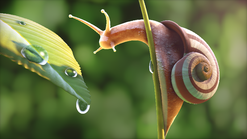
… Or make beautiful photo realistic images and videos which render in real time.
Snail by Inigo Quilez https://www.shadertoy.com/view/ld3Gz2
Shadertoy was founded by demosceners which are people that have parties & competitions to make very small executables that generate impressive audio and visuals.
Besides demosceners, shadertoy.com is frequented by professional and hobbyist game developers, graphics researchers, people who work in movies, and all sorts of other people as well.
It’s a great place to play and learn because it lets you dive in without a lot of fuss. I have learned so much there it boggles my mind sometimes… all sorts of math tricks, graphics techniques, dual numbers for automatic differentiation, ray marching solid geometry, and I even did real time ray tracing back in 2013. Real time ray tracing may SEEM new to the world, but demo sceners are doing real time ray tracing on things like the comodore 64 and have been doing so for years or decades. The rest of us are just catching up!
In these articles we are going to be doing path tracing in shadertoy because it’s very easy to do so. You should head over there, create an account and look around a bit at some of the shadertoys. Shadertoy works best in chrome or firefox.
We’ll get started when you come back 🙂
New Shader
To get started, after you log in, click on the “new” button in the upper right to create a new shader. You should be greeted by something that looks like this:
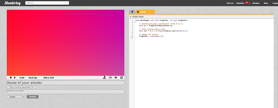
Go ahead and give the shader a name – the names must be globally unique! – as well as at least one tag, and a description. All of those are required so that you can click “Submit” and do the initial save for your shader.
After you have submitted your shader, the submit button will turn into a save button, and you will be good to go onto the next step.
Generating Rays
Path tracing is a type of ray tracing, which means we are going to shoot a ray into the world out of every pixel. For each individual ray, we are going to see what it hits and use that information to give a color to our pixel. Doing that for every pixel independently gives us our final image.
So, the first step to doing path tracing is to calculate the rays for each pixel. A ray has a starting point and a direction, so we are going to need to calculate where the ray starts, and what direction it is going in.
The ray is going to start at the camera location (you could think of this as the eye location), and it’s going to shoot at pixels on an imaginary rectangle in front of the camera, go through those pixels, and go out into the scene to see what they hit.
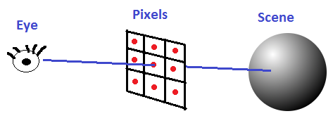
We are going to make this rectangle of pixels be from -1 to +1 on the x and y axis, and for now we’ll make it be 1 unit away on the z axis. We’ll say the camera is at the origin (0,0,0). Our goal is to calculate the 3d point on this rectangle for each pixel, then calculate the direction of the ray from the origin to that 3d point.
We’ll start by calculating each pixel’s percentage on the x and y axis from 0 to 1. We’ll show that in the red and green channel to make sure we are doing it correctly.
Put this code below in the code box in the right and click the play button (circled red in the screenshot) to see the results.
void mainImage( out vec4 fragColor, in vec2 fragCoord )
{
    // calculate pixel coordinates as a percetange of the screen, from 0 to 1 on each axis
    vec2 uv = fragCoord/iResolution.xy;

    // show percentage as red and green
    fragColor = vec4(uv, 0.0f, 1.0f);
}
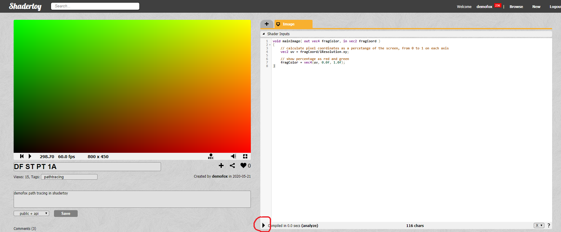
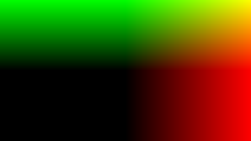
We can see from this picture that (0,0) is in the lower left, where the color is black. As the pixels go to the right, they get more red, which shows us that the x axis goes to the right. As the pixels go up, they get more green, which shows us that the y axis goes upward.
Visualizing values like this is a great way to debug shadertoy shaders. The usual graphics debuggers and debugging techniques are not available when doing webgl, or when using shadertoy, so this “printf” style debugging is the best way to see what’s going on if you are having problems.
Now that we have screen percentage from 0 to 1, we want to change it to being from -1 to 1 so that it’s actually just the x and y coordinate on the imaginary pixel rectangle.
void mainImage( out vec4 fragColor, in vec2 fragCoord )
{
    // calculate 2d coordinates of the ray target on the imaginary pixel plane.
    // -1 to +1 on each axis.
    vec2 pixelTarget2D = (fragCoord/iResolution.xy) * 2.0f - 1.0f;

    // show percentage as red and green
    fragColor = vec4(pixelTarget2D, 0.0f, 1.0f);
}
We can see now that it’s black in the middle of the screen, and going to the right makes the pixels more red while going up makes the pixels more green. However, going left and down doesn’t change the color at all and just leaves it black. This is because colors are clamped to be between 0 and 1 before being displayed, making all negative numbers just be zero.
if you wanted to make sure the negative values were down there, and it really wasn’t just zero, you could visualize the absolute value like this.
void mainImage( out vec4 fragColor, in vec2 fragCoord )
{
    // calculate 2d coordinates of the ray target on the imaginary pixel plane.
    // -1 to +1 on each axis.
    vec2 pixelTarget2D = (fragCoord/iResolution.xy) * 2.0f - 1.0f;

    // take absolute value of the pixel target so we can verify there are negative values in the lower left.
    pixelTarget2D = abs(pixelTarget2D);

    // show percentage as red and green
    fragColor = vec4(pixelTarget2D, 0.0f, 1.0f);
}

Ok so now we have the x,y location of the ray target on the imaginary pixel rectangle. We can make the z location be 1 since we want it to be 1 unit away, and that gives us a target for our ray. We now want to get a NORMALIZED vector from the camera position (the origin) to this ray target. That gives us our ray direction and we can visualize that ray to verify that it looks somewhat reasonable.
void mainImage( out vec4 fragColor, in vec2 fragCoord )
{
    // The ray starts at the camera position (the origin)
    vec3 rayPosition = vec3(0.0f, 0.0f, 0.0f);

    // calculate coordinates of the ray target on the imaginary pixel plane.
    // -1 to +1 on x,y axis. 1 unit away on the z axis
    vec3 rayTarget = vec3((fragCoord/iResolution.xy) * 2.0f - 1.0f, 1.0f);

    // calculate a normalized vector for the ray direction.
    // it's pointing from the ray position to the ray target.
    vec3 rayDir = normalize(rayTarget - rayPosition);

    // show the ray direction
    fragColor = vec4(rayDir, 1.0f);
}
it’s a little subtle, but as you go right from the center of the screen, the pixels get more red and become a purpleish color. As you go up from the center, the pixels get more green and become a little more teal. This shows us that our ray directions seem sensible. As we move right on the x axis, the normalized ray direction also starts deviating from straight ahead and points more to the right, more positively on the x axis. Similarly for the y axis and the green color.
Going left and down from center, the blue gets darker, but no red and green show up due to the x and y axis being negative values again.
If you play around with the z coordinate of the ray target, you can make the ray direction changes more or less obvious due to basically zooming in or out the camera by moving the imaginary pixel rectangle, but we’ll talk more about that in a little bit.
The nearly constant blue color on the screen is due to the positive z value of the ray direction. All of the rays are aiming forward, which is what we’d expect.
We have successfully calculated a ray starting position and direction, and are ready to start shooting rays into the world!
Rendering Geometry
Next we want to use these rays to actually render some geometry. To do this we need functions that will tell us whether a ray intersects a shape or not, and how far down the ray the intersection happens.
We are going to use the functions “TestSphereTrace” and “TestQuadTrace” for ray intersection vs sphere, and ray intersection vs rectangle (quad). Apologies for not having them in a copy/pastable format here in the post. WordPress malfunctions when I try to put them into a code block, but they are in the final shader toy.
There are other ray vs object intersection functions that you can find. I adapted these from Christer Ericson’s book “Real-Time Collision Detection” (https://www.amazon.com/Real-Time-Collision-Detection-Interactive-Technology/dp/1558607323), and there a bunch on the net if you google for them. Ray marching can also be used as a numerical method for ray vs object intersection, which lets you have much richer shapes, infinitely repeating objects, and more.
Anyhow, instead of using the ray direction for the color for each pixel, we are going to test the ray against a scene made up of multiple objects, and give a different color to each object. We do that in the GetColorForRay function.
// The minimunm distance a ray must travel before we consider an intersection.
// This is to prevent a ray from intersecting a surface it just bounced off of.
const float c_minimumRayHitTime = 0.1f;
// the farthest we look for ray hits
const float c_superFar = 10000.0f;
struct SRayHitInfo
{
float dist;
vec3 normal;
};
float ScalarTriple(vec3 u, vec3 v, vec3 w)
{
return dot(cross(u, v), w);
}
bool TestQuadTrace(in vec3 rayPos, in vec3 rayDir, inout SRayHitInfo info, in vec3 a, in vec3 b, in vec3 c, in vec3 d)
{
// ...
}
bool TestSphereTrace(in vec3 rayPos, in vec3 rayDir, inout SRayHitInfo info, in vec4 sphere)
{
// ...
}
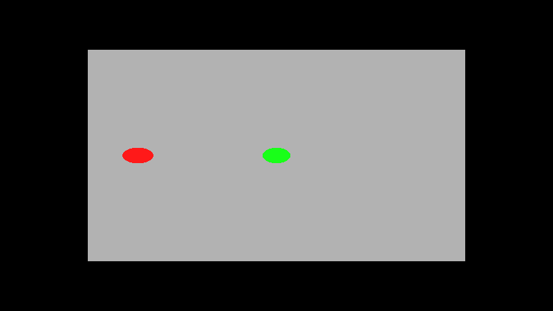
vec3 GetColorForRay(in vec3 rayPos, in vec3 rayDir)
{
SRayHitInfo hitInfo;
hitInfo.dist = c_superFar;
vec3 ret = vec3(0.0f, 0.0f, 0.0f);
if (TestSphereTrace(rayPos, rayDir, hitInfo, vec4(-10.0f, 0.0f, 20.0f, 1.0f)))
{
ret = vec3(1.0f, 0.1f, 0.1f);
}
if (TestSphereTrace(rayPos, rayDir, hitInfo, vec4(0.0f, 0.0f, 20.0f, 1.0f)))
{
ret = vec3(0.1f, 1.0f, 0.1f);
}
{
vec3 A = vec3(-15.0f, -15.0f, 22.0f);
vec3 B = vec3( 15.0f, -15.0f, 22.0f);
vec3 C = vec3( 15.0f, 15.0f, 22.0f);
vec3 D = vec3(-15.0f, 15.0f, 22.0f);
if (TestQuadTrace(rayPos, rayDir, hitInfo, A, B, C, D))
{
ret = vec3(0.7f, 0.7f, 0.7f);
}
}
if (TestSphereTrace(rayPos, rayDir, hitInfo, vec4(10.0f, 0.0f, 20.0f, 1.0f)))
{
ret = vec3(0.1f, 0.1f, 1.0f);
}
return ret;
}
void mainImage( out vec4 fragColor, in vec2 fragCoord )
{
// The ray starts at the camera position (the origin)
vec3 rayPosition = vec3(0.0f, 0.0f, 0.0f);
// calculate coordinates of the ray target on the imaginary pixel plane.
// -1 to +1 on x,y axis. 1 unit away on the z axis
vec3 rayTarget = vec3((fragCoord/iResolution.xy) * 2.0f - 1.0f, 1.0f);
// calculate a normalized vector for the ray direction.
// it's pointing from the ray position to the ray target.
vec3 rayDir = normalize(rayTarget - rayPosition);
// raytrace for this pixel
vec3 color = GetColorForRay(rayPosition, rayDir);
// show the result
fragColor = vec4(color, 1.0f);
}

We see some things on the screen which is nice, but we have a ways to go yet before we are path tracing.
If you look at the code in the final shadertoy, TestSphereTrace and TestQuadTrace only return true if the ray intersects with the shape AND the intersection distance is closer than hitInfo.dist. A common mistake to make when first doing any kind of raytracing (path tracing or other types) is to accept the first thing a ray hits, but you actually want to test all objects and keep whichever hit is closest.
If you only kept the first hit found, not the closest hit, the blue ball would disappear, because the ray test for the grey quad comes before the blue ball, even though it’s farther away.
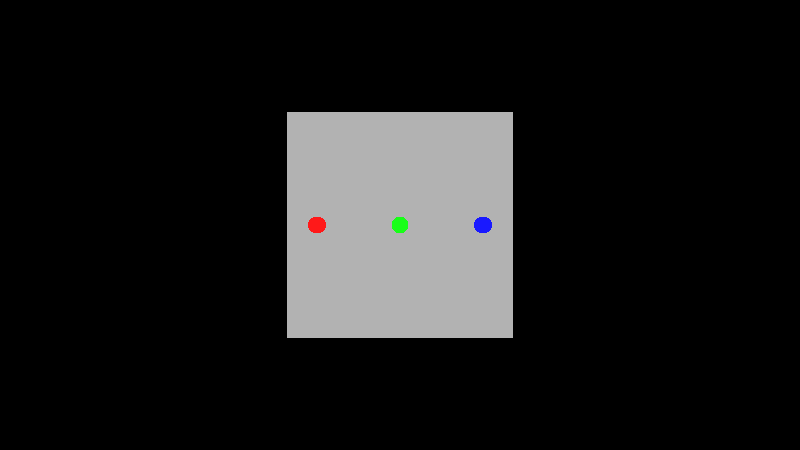
Correcting Aspect Ratio
You probably noticed that the spheres were stretched in the last image. The reason for that is that our imaginary pixel rectangle is a square (it’s from -1 to +1 on the x and y axis), while the image we are rendering is not a square. That makes the image get stretched horizontally.
The way to fix this is to either grow the imaginary pixel rectangle on the x axis, or shrink it on the y axis, so that the ratio of the width to the height is the same on the imaginary pixel rectangle as it is in our rendered image. I’m going to shrink the y axis. Here is the new mainImage function to use. Lines 10 through 12 were added to fix the problem.
void mainImage( out vec4 fragColor, in vec2 fragCoord )
{
    // The ray starts at the camera position (the origin)
    vec3 rayPosition = vec3(0.0f, 0.0f, 0.0f);

    // calculate coordinates of the ray target on the imaginary pixel plane.
    // -1 to +1 on x,y axis. 1 unit away on the z axis
    vec3 rayTarget = vec3((fragCoord/iResolution.xy) * 2.0f - 1.0f, 1.0f);

    // correct for aspect ratio
	float aspectRatio = iResolution.x / iResolution.y;
    rayTarget.y /= aspectRatio;

    // calculate a normalized vector for the ray direction.
    // it's pointing from the ray position to the ray target.
    vec3 rayDir = normalize(rayTarget - rayPosition);

    // raytrace for this pixel
    vec3 color = GetColorForRay(rayPosition, rayDir);

    // show the result
    fragColor = vec4(color, 1.0f);
}

Camera Zoom (FOV)
I said before that the imaginary pixel rectangle would be 1 unit away, but if we make that distance smaller, it’s the same as zooming the camera out or increasing the field of view. If we make that distance larger, it’s the same as zooming the camera in or decreasing the field of view.
It turns out that having the pixel rectangle be 1 unit away gives you a field of view of 90 degrees.
The formula for calculating the distance for a specific field of view is on line 7 of the new mainImage function below and is used on line 11.
void mainImage( out vec4 fragColor, in vec2 fragCoord )
{
    // The ray starts at the camera position (the origin)
    vec3 rayPosition = vec3(0.0f, 0.0f, 0.0f);

    // calculate the camera distance
	float cameraDistance = 1.0f / tan(c_FOVDegrees * 0.5f * c_pi / 180.0f);

    // calculate coordinates of the ray target on the imaginary pixel plane.
    // -1 to +1 on x,y axis. 1 unit away on the z axis
    vec3 rayTarget = vec3((fragCoord/iResolution.xy) * 2.0f - 1.0f, cameraDistance);

    // correct for aspect ratio
	float aspectRatio = iResolution.x / iResolution.y;
    rayTarget.y /= aspectRatio;

    // calculate a normalized vector for the ray direction.
    // it's pointing from the ray position to the ray target.
    vec3 rayDir = normalize(rayTarget - rayPosition);

    // raytrace for this pixel
    vec3 color = GetColorForRay(rayPosition, rayDir);

    // show the result
    fragColor = vec4(color, 1.0f);
}
We are going to leave c_FOVDegrees at 90 degrees as we move forward, but here it is at 120 degrees
and here it is at 45 degrees
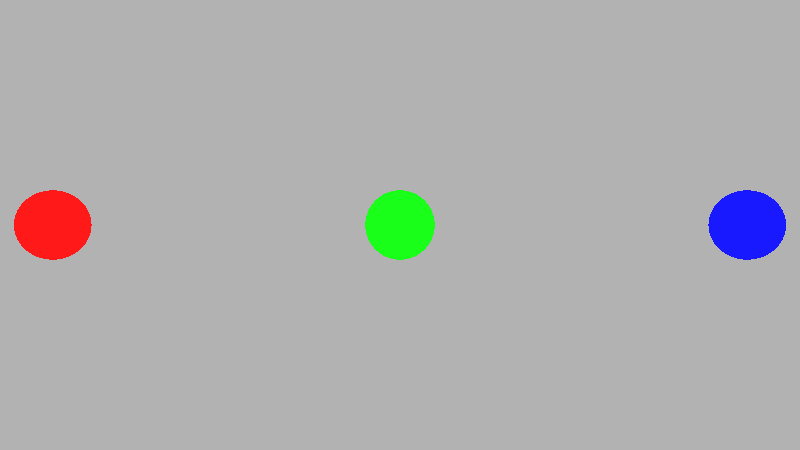
If you make the FOV too wide, you’ll start getting distortion at the edges. That’s a deep topic that cameras experience too that we won’t go into but I wanted to make sure you knew about that. You can get some real interesting renders by setting the FOV to really large values like 360 or 720 degrees!
Let’s Path Trace!
Now that we can shoot rays into the world, we are finally ready to do some path tracing!
To do shading we’ll need light sources, and our light sources will just be objects that have emissive lighting, aka glowing objects.
For this post we are only going to do diffuse light shading, which means no shiny reflections. We’ll do shiny reflections probably in the very next post in this series, but for now we’ll just do diffuse.
So, objects will have two fields that define their material:
- a vec3 for emissive, specifying how much they glow in RGB
- a vec3 for albedo, specifying what color they are under white light
How path tracing works in this setup is pretty simple. We’ll start out a pixel’s color at black, a “throughput” color at white, and we’ll shoot a ray out into the world, obeying the following rules:
- When a ray hits an object, emissive*throughput is added to the pixel’s color.
- When a ray hits an object, the throughput is multiplied by the object’s albedo, which affects the color of future emissive lights.
- When a ray hits an object, a ray will be reflected in a random direction and the ray will continue (more info in a sec)
- We will terminate when a ray misses all objects, or when N ray bounces have been reached. (N=8 in this shadertoy, but you can tune that value for speed vs correctness)
That is all there is to it!
The concept of “throughput” might seem strange at first but think of these scenarios as they increase in complexity:
- A ray hits a white ball, bounces off and hits a white light. The pixel should be white, because the white ball is lit by white light.
- A ray hits a red ball, bounces off and hits the same white light. The pixel should be red because red ball is lit by white light.
- A ray hits a white ball, bounces off and hits a red ball, bounces off and hits a white light. The pixel should be red because the white ball is lit by the red ball being lit by the white light.
When a ray bounces off a surface, all future lighting for that ray is multiplied by the color of that surface.
These simple rules are all you need to get soft shadows, bounce lighting, ambient occlusion, and all the rest of the cool things you see show up “automagically” in path tracers.
I said that the ray bounces off randomly but there are two different ways to handle this:
- Bounce randomly in the positive hemisphere of the normal and then multiply throughput by dot(newRayDir, surfaceNormal). This is the cosine theta term for diffuse lighting.
- Or, bounce randomly in a cosine weighted hemisphere direction of the surface normal. This uses importance sampling for the cosine theta term and is the better way to go.
To do #2, all we need to do is get a “random point on sphere” (also known as a random unit vector), add it to the normal, and normalize the result. It’s nice how simple it is.
You are probably wondering how to generate random numbers in a shader. There are many ways to handle it, but here’s how we are going to do it.
First, we are going to initialize a random seed for the current pixel, based on pixel position and frame number, so that each pixel gets different random numbers, and also so that each pixel gets different random numbers each frame.
We can just put this at the top of our mainImage function:
    // initialize a random number state based on frag coord and frame
    uint rngState = uint(uint(fragCoord.x) * uint(1973) + uint(fragCoord.y) * uint(9277) + uint(iFrame) * uint(26699)) | uint(1);
Then, we can toss these functions above our mainImage function, which take the rngState in, modify it, and generate a random number.
uint wang_hash(inout uint seed)
{
    seed = uint(seed ^ uint(61)) ^ uint(seed >> uint(16));
    seed *= uint(9);
    seed = seed ^ (seed >> 4);
    seed *= uint(0x27d4eb2d);
    seed = seed ^ (seed >> 15);
    return seed;
}

float RandomFloat01(inout uint state)
{
    return float(wang_hash(state)) / 4294967296.0;
}

vec3 RandomUnitVector(inout uint state)
{
    float z = RandomFloat01(state) * 2.0f - 1.0f;
    float a = RandomFloat01(state) * c_twopi;
    float r = sqrt(1.0f - z * z);
    float x = r * cos(a);
    float y = r * sin(a);
    return vec3(x, y, z);
}
To implement the path tracing rules we previously described, we are going to change some things…
- Move the ray vs object tests from GetColorForRay into a new function called TestSceneTrace. This lets us separate the scene testing logic from the iterative bounce raytracing we are going to do.
- Add albedo and emissive vec3’s to hit info and set both fields whenever we intersect an object. This is the object material data.
- Implement iterative raytracing in GetColorForRay as we described it
- Add a light to the scene so it isn’t completely dark
void TestSceneTrace(in vec3 rayPos, in vec3 rayDir, inout SRayHitInfo hitInfo)
{
    {
        vec3 A = vec3(-15.0f, -15.0f, 22.0f);
        vec3 B = vec3( 15.0f, -15.0f, 22.0f);
        vec3 C = vec3( 15.0f,  15.0f, 22.0f);
        vec3 D = vec3(-15.0f,  15.0f, 22.0f);
        if (TestQuadTrace(rayPos, rayDir, hitInfo, A, B, C, D))
        {
            hitInfo.albedo = vec3(0.7f, 0.7f, 0.7f);
            hitInfo.emissive = vec3(0.0f, 0.0f, 0.0f);
        }
	}

	if (TestSphereTrace(rayPos, rayDir, hitInfo, vec4(-10.0f, 0.0f, 20.0f, 1.0f)))
    {
        hitInfo.albedo = vec3(1.0f, 0.1f, 0.1f);
        hitInfo.emissive = vec3(0.0f, 0.0f, 0.0f);
    }

	if (TestSphereTrace(rayPos, rayDir, hitInfo, vec4(0.0f, 0.0f, 20.0f, 1.0f)))
    {
        hitInfo.albedo = vec3(0.1f, 1.0f, 0.1f);
        hitInfo.emissive = vec3(0.0f, 0.0f, 0.0f);
    }

	if (TestSphereTrace(rayPos, rayDir, hitInfo, vec4(10.0f, 0.0f, 20.0f, 1.0f)))
    {
        hitInfo.albedo = vec3(0.1f, 0.1f, 1.0f);
        hitInfo.emissive = vec3(0.0f, 0.0f, 0.0f);
    }


	if (TestSphereTrace(rayPos, rayDir, hitInfo, vec4(10.0f, 10.0f, 20.0f, 5.0f)))
    {
        hitInfo.albedo = vec3(0.0f, 0.0f, 0.0f);
        hitInfo.emissive = vec3(1.0f, 0.9f, 0.7f) * 100.0f;
    }
}

vec3 GetColorForRay(in vec3 startRayPos, in vec3 startRayDir, inout uint rngState)
{
    // initialize
    vec3 ret = vec3(0.0f, 0.0f, 0.0f);
    vec3 throughput = vec3(1.0f, 1.0f, 1.0f);
    vec3 rayPos = startRayPos;
    vec3 rayDir = startRayDir;

    for (int bounceIndex = 0; bounceIndex <= c_numBounces; ++bounceIndex)
    {
        // shoot a ray out into the world
        SRayHitInfo hitInfo;
        hitInfo.dist = c_superFar;
        TestSceneTrace(rayPos, rayDir, hitInfo);

        // if the ray missed, we are done
        if (hitInfo.dist == c_superFar)
            break;

		// update the ray position
        rayPos = (rayPos + rayDir * hitInfo.dist) + hitInfo.normal * c_rayPosNormalNudge;

        // calculate new ray direction, in a cosine weighted hemisphere oriented at normal
        rayDir = normalize(hitInfo.normal + RandomUnitVector(rngState));

		// add in emissive lighting
        ret += hitInfo.emissive * throughput;

        // update the colorMultiplier
        throughput *= hitInfo.albedo;
    }

    // return pixel color
    return ret;
}

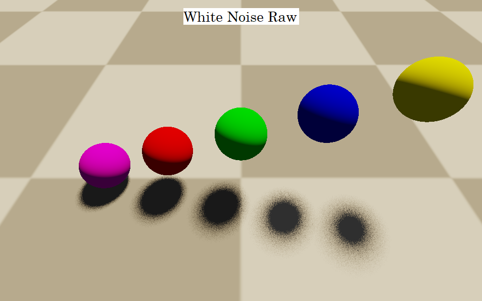
When we run the shadertoy we see something like the above, but the specific dots we see move around each frame due to being random over time.
This might not look great but we are really close now. We just need to make pixels show their average value instead of only a single value.
Averaging Pixel Values
To average the pixel values We are going to need to make our shader into a multipass shader.
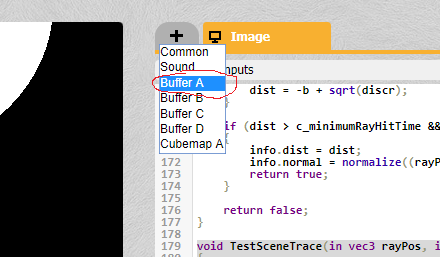
The first step is to make another pass. Click the + sign next to the “image” tab and select “Buffer A”
Now you should have a Buf A tab next to the image tab.
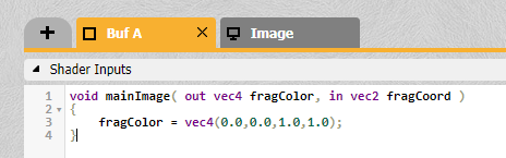
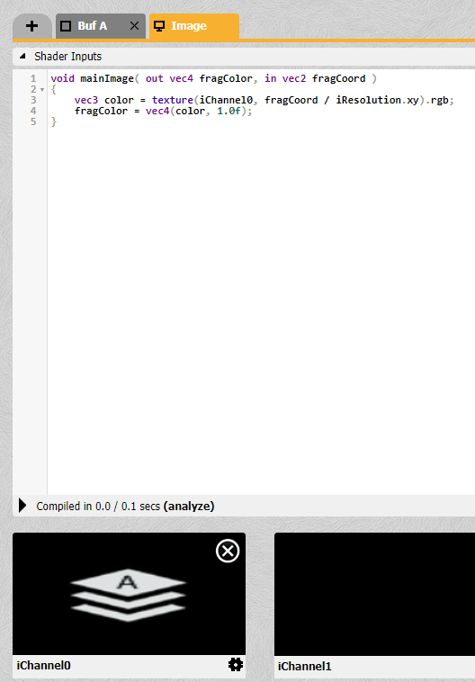
Move everything from the image tab to the Buf A tab. In the image tab, select “Buffer A” for texture “iChannel0” and put this code in to read and show pixels from Buffer A.
void mainImage( out vec4 fragColor, in vec2 fragCoord )
{
    vec3 color = texture(iChannel0, fragCoord / iResolution.xy).rgb;
    fragColor = vec4(color, 1.0f);
}
The next step is to actually average the pixel values.
In the “Buf A” tab, also select “Buffer A” for texture “iChannel0” so that we can read Buffer A’s pixel from last frame, to average into the current frame’s output. Now we just add lines 27, 28, 29 below to average all the pixels together!
void mainImage( out vec4 fragColor, in vec2 fragCoord )
{
    // initialize a random number state based on frag coord and frame
    uint rngState = uint(uint(fragCoord.x) * uint(1973) + uint(fragCoord.y) * uint(9277) + uint(iFrame) * uint(26699)) | uint(1);

    // The ray starts at the camera position (the origin)
    vec3 rayPosition = vec3(0.0f, 0.0f, 0.0f);

    // calculate the camera distance
	float cameraDistance = 1.0f / tan(c_FOVDegrees * 0.5f * c_pi / 180.0f);

    // calculate coordinates of the ray target on the imaginary pixel plane.
    // -1 to +1 on x,y axis. 1 unit away on the z axis
    vec3 rayTarget = vec3((fragCoord/iResolution.xy) * 2.0f - 1.0f, cameraDistance);

    // correct for aspect ratio
	float aspectRatio = iResolution.x / iResolution.y;
    rayTarget.y /= aspectRatio;

    // calculate a normalized vector for the ray direction.
    // it's pointing from the ray position to the ray target.
    vec3 rayDir = normalize(rayTarget - rayPosition);

    // raytrace for this pixel
    vec3 color = GetColorForRay(rayPosition, rayDir, rngState);

    // average the frames together
    vec3 lastFrameColor = texture(iChannel0, fragCoord / iResolution.xy).rgb;
    color = mix(lastFrameColor, color, 1.0f / float(iFrame+1));

    // show the result
    fragColor = vec4(color, 1.0f);
}

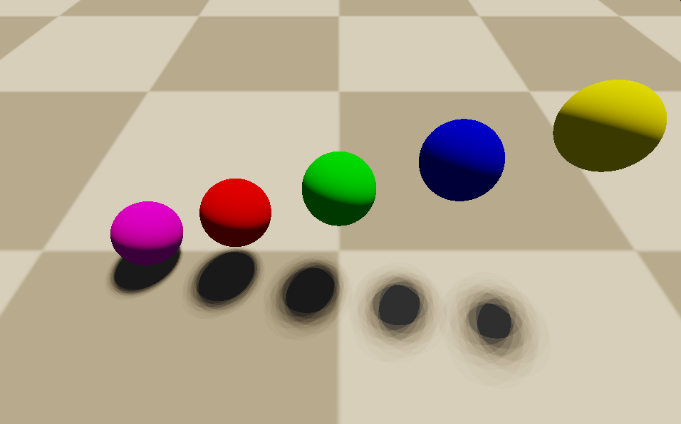
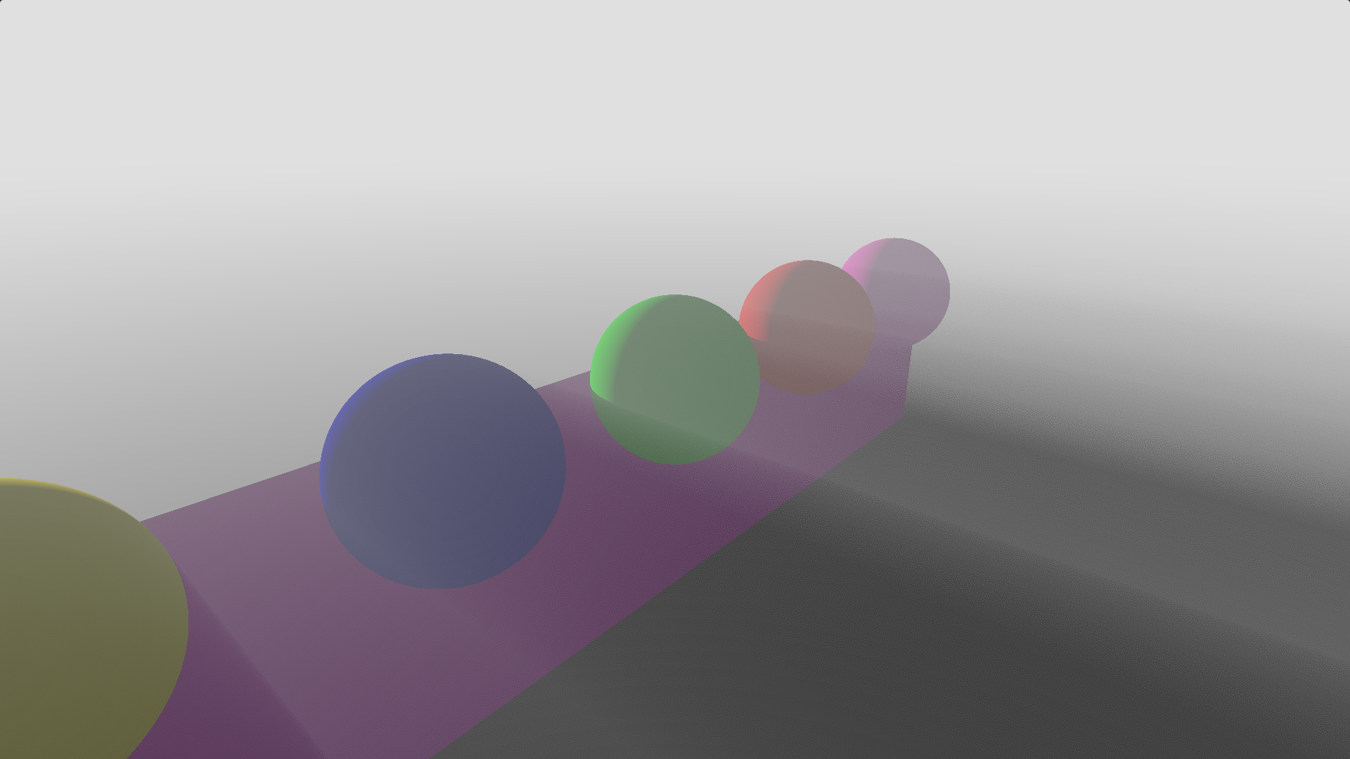
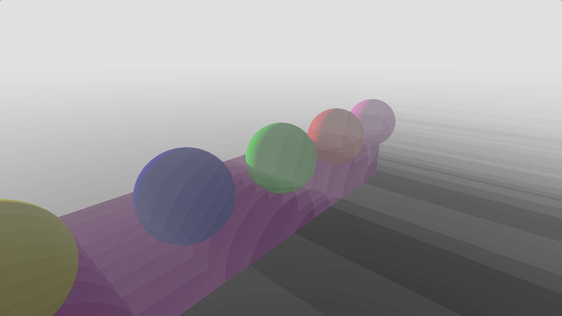
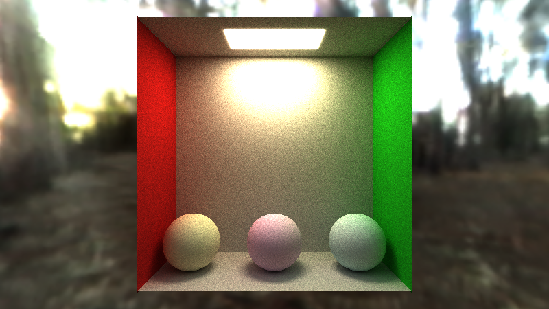
After 5 minutes of rendering, the result looks pretty noisy, pixels are too bright and clip, and it isn’t a great scene, but we are in fact path tracing now! You can even see some neat lighting effects, like how you see some red on the wall next to the red ball, due to light reflecting off of it. The spheres are casting some nice looking shadows too.
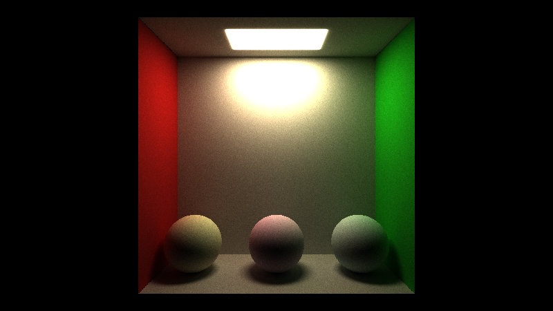
We can clean up the scene a little bit, make something like a cornell box and get this render after 5 minutes
When Rays Miss
One last feature before we close up this first post in the series.
Right now when a ray misses the scene and flies out into the void, we stop raytracing, which implicitly is saying that the void outside the scene is black. Instead of having our background be black, let’s have it be an environment.
In the “Buf A” tab choose the forest cube map for texture iChannel1 and then add line 19 to GetColorForRay() below.
vec3 GetColorForRay(in vec3 startRayPos, in vec3 startRayDir, inout uint rngState)
{
    // initialize
    vec3 ret = vec3(0.0f, 0.0f, 0.0f);
    vec3 throughput = vec3(1.0f, 1.0f, 1.0f);
    vec3 rayPos = startRayPos;
    vec3 rayDir = startRayDir;

    for (int bounceIndex = 0; bounceIndex <= c_numBounces; ++bounceIndex)
    {
        // shoot a ray out into the world
        SRayHitInfo hitInfo;
        hitInfo.dist = c_superFar;
        TestSceneTrace(rayPos, rayDir, hitInfo);

        // if the ray missed, we are done
        if (hitInfo.dist == c_superFar)
        {
            ret += texture(iChannel1, rayDir).rgb * throughput;
            break;
        }

		// update the ray position
        rayPos = (rayPos + rayDir * hitInfo.dist) + hitInfo.normal * c_rayPosNormalNudge;

        // calculate new ray direction, in a cosine weighted hemisphere oriented at normal
        rayDir = normalize(hitInfo.normal + RandomUnitVector(rngState));

		// add in emissive lighting
        ret += hitInfo.emissive * throughput;

        // update the colorMultiplier
        throughput *= hitInfo.albedo;
    }

    // return pixel color
    return ret;
}
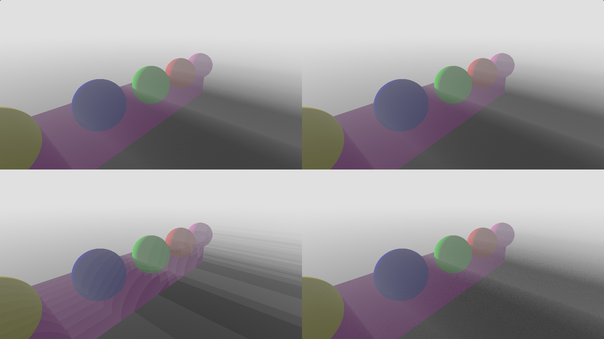
With those changes, here is a 30 second render.
Noise
In 30 seconds it looks about as noisy as the previous 5 minute render did. The 5 minute render looks so much worse because the scene has both very dark places and very bright places. The more different the lighting conditions are in different places in a scene, the more noise you will have. Also, smaller brighter lights will cause more noise than larger dimmer lights.
Learning more sophisticated path tracing techniques (like direct light sampling, also known as next event estimation) makes this not be true, but we are aiming for understandability in this path tracer, not convergence speed.
But, you might notice that as your scene is rendering, shadertoy is reporting 60fps, meaning that the scene rendering is being limited by vsync. The rendering would go faster than 60fps if it could, and so would converge faster, but it can’t.
There’s a shadertoy plugin for chrome that you can install to help this, and you can tell it to do up to 64 draws per frame, which really helps it converge more quickly. I’m on a ~5 year old gaming laptop with an nvidia 980m gpu in it, and I got this full screen render in a minute, which has converged pretty nicely! Click on it to view it full screen.
You can get the shadertoy plugin here: https://chrome.google.com/webstore/detail/shadertoy-unofficial-plug/ohicbclhdmkhoabobgppffepcopomhgl
An alternative to getting the shadertoy plugin for chrome is to just shoot N rays out for the pixel each frame, and average them, before putting them into the averaged buffer. That is more efficient than doing the multiple shader passes N times a frame since things are in the memory cache etc when iterating inside the shader. That means your image will converge more in the same amount of time.
Closing
The shadertoy that made this image, that contains everything talked about in this post, is at: https://www.shadertoy.com/view/tsBBWW
Try playing around with the path tracer, making a different scene, and modifying the code for other visual effects.
If you make something, I’d love to see it! You can find me on twitter at @Atrix256
There are going to be 3 or 4 more posts in this series that will be coming pretty quickly, on a variety of topics including depth of field and bokeh, shiny reflections, anti aliasing and fog/smoke. We also are not even sRGB correct yet! These things will improve the image significantly so stay tuned.
Some other awesome resources regarding path tracing are:
- Peter Shirley’s “Ray Tracing in One Weekend” (now a free PDF) https://www.realtimerendering.com/raytracing/Ray%20Tracing%20in%20a%20Weekend.pdf
- Morgan McGuire’s “Graphics Codex” https://graphicscodex.com/
- My more formal blog post on diffuse & emissive path tracing https://blog.demofox.org/2016/09/21/path-tracing-getting-started-with-diffuse-and-emissive/
Path tracing doesn’t only have to be used for realistic rendering though. Below is a stylized path tracing shadertoy I made, in vaporwave style.
“Neon Desert” stylize path tracer shadertoy: https://www.shadertoy.com/view/tdXBW8
Thanks for reading, part 2 coming soon!