In basic algebra we were taught that if we have three unknowns (variables), it takes three equations to solve for them.

There’s some fine print though that isn’t talked about until quite a bit later.

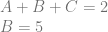
Let’s have a look at three unknowns in two equations:

If we just need a third equation to solve this, why not just modify the second equation to make a third?

That obviously doesn’t work, because it doesn’t add any new information! If you try it out, you’ll find that adding that equation doesn’t get you any closer to solving for the variables.

So, it takes three equations to solve for three unknowns, but the three equations have to provide unique, meaningful information. That is the fine print.

How can we know if an equation provides unique, meaningful information though?

It turns out that linear algebra gives us a neat technique for simplifying a system of equations. It actually solves for individual variables if it’s able to, and also gets rid of redundant equations that don’t add any new information.

This simplest form is called the Reduced Row Echelon Form (Wikipedia) which you may also see abbreviated as “rref” (perhaps a bit of a confusing term for programmers) and it involves you putting the equations into a matrix and then performing an algorithm, such as Gauss–Jordan elimination (Wikipedia) to get the rref.

Equations as a Matrix

Putting n set of equations into a matrix is really straight forward.

Each row of a matrix is a separate equation, and each column represents the coefficient of a variable.

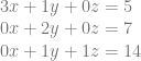
Let’s see how with this set of equations:

Not every equation has every variable in it, so let’s fix that by putting in zero terms for the missing variables, and let’s make the one terms explicit as well:

Putting those equations into a matrix looks like this:

If you also include the constants on the right side of the equation, you get what is called an augmented matrix, which looks like this:

Reduced Row Echelon Form

Wikipedia explains the reduced row echelon form this way:

• all nonzero rows (rows with at least one nonzero element) are above any rows of all zeroes (all zero rows, if any, belong at the bottom of the matrix), and
• the leading coefficient (the first nonzero number from the left, also called the pivot) of a nonzero row is always strictly to the right of the leading coefficient of the row above it.
• Every leading coefficient is 1 and is the only nonzero entry in its column.

This is an example of a 3×5 matrix in reduced row echelon form:

Basically, the lower left triangle of the matrix (the part under the diagonal) needs to be zero, and the first number in each row needs to be one.

Looking back at the augmented matrix we made:

If we put it into reduced row echelon form, we get this:

There’s something really neat about the reduced row echelon form. If we take the above augmented matrix and turn it back into equations, look what we get:

Or if we simplify that:

Putting it into reduced row echelon form simplified our set of equations so much that it actually solved for our variables. Neat!

How do we put a matrix into rref? We can use Gauss–Jordan elimination.

Gauss–Jordan Elimination

Gauss Jordan Elimination is a way of doing operations on rows to be able to manipulate the matrix to get it into the desired form.

It’s often explained that there are three row operations you can do:

• Type 1: Swap the positions of two rows.
• Type 2: Multiply a row by a nonzero scalar.
• Type 3: Add to one row a scalar multiple of another.

You might notice that the first two rules are technically just cases of using the third rule. I find that easier to remember, maybe you will too.

The algorithm for getting the rref is actually pretty simple.

1. Starting with the first column of the matrix, find a row which has a non zero in that column, and make that row be the first row by swapping it with the first row.
2. Multiply the first row by a value so that the first column has a 1 in it.
3. Subtract a multiple of the first row from every other row in the matrix so that they have a zero in the first column.

You’ve now handled one column (one variable) so move onto the next.

1. Continuing on, we consider the second column. Find a row which has a non zero in that column and make that row be the second row by swapping it with the second row.
2. Multiply the second row by a value so that the second column has a 1 in it.
3. Subtract a multiple of the second row from every other row in the matrix so that they have a zero in the second column.

You repeat this process until you either run out of rows or columns, at which point you are done.

Note that if you ever find a column that has only zeros in it, you just skip that row.

Let’s work through the example augmented matrix to see how we got it into rref. Starting with this:

We already have a non zero in the first column, so we multiply the top row by 1/3 to get this:

All the other rows have a zero in the first column so we move to the second row and the second column. The second row already has a non zero in the second column, so we multiply the second row by 1/2 to get this:

To make sure the second row is the only row that has a non zero in the second column, we subtract the second row times 1/3 from the first row. We also subtract the second row from the third row. That gives us this:

Since the third row has a 1 in the third column, and all other rows have a 0 in that column we are done.

That’s all there is to it! We put the matrix into rref, and we also solved the set of equations. Neat huh?

You may notice that the ultimate rref of a matrix is just the identity matrix. This is true unless the equations can’t be fully solved.

Overdetermined, Underdetermined & Inconsistent Equations

Systems of equations are overdetermined when they have more equations than unknowns, like the below which has three equations and two unknowns:

Putting that into (augmented) matrix form gives you this:

If you put that into rref, you end up with this:

The last row became zeroes, which shows us that there was redundant info in the system of equations that disappeared. We can easily see that x = 1 and y = 2, and that satisfies all three equations.

Just like we talked about in the opening of this post, if you have equations that don’t add useful information beyond what the other equations already give, it will disappear when you put it into rref. That made our over-determined system become just a determined system.

What happens though if we change the third row in the overdetermined system to be something else? For instance, we can say y=10 instead of y=2:

The augmented matrix for that is this:

If we put that in rref, we get the identity matrix out which seems like everything is ok:

However, if we turn it back into a set of equations, we can see that we have a problem:

The result says that 0 = 1, which is not true. Having a row of “0 = 1” in rref is how you detect that a system of equations is inconsistent, or in other words, that the equations give contradictory information.

A system of equations can also be underderdetermined, meaning there isn’t enough information to solve the equations. Let’s use the example from the beginning of the post:

In an augmented matrix, that looks like this:

Putting that in rref we get this:

Converting the matrix back into equations we get this:

This says there isn’t enough information to fully solve the equations, and shows how A and C are related, even though B is completely determined.

Note that another way of looking at this is that “A” and “C” are “free variables”. That means that if your equations specify constraints, that you are free to choose a value for either A or C. If you choose a value for one, the other becomes defined. B is not a free variable because it’s value is determined.

Let’s finish the example from the beginning of the post, showing what happens when we “make up” an equation by transforming one of the equations we already have:

The augmented matrix looks like this:

Putting it in rref, we get this:

Which as you can see, our rref matrix is the same as it was without the extra “made up” equation besides the extra row of zeros in the result.

The number of non zero rows in a matrix in rref is known as the rank of the matrix. In these last two examples, the rank of the matrix was two in both cases. That means that you can tell if adding an equation to a system of equations adds any new, meaningful information or not by seeing if it changes the rank of the matrix for the set of equations. If the rank is the same before and after adding the new equation, it doesn’t add anything new. If the rank does change, that means it does add new information.

This concept of “adding new, meaningful information” actually has a formalized term: linear independence. If a new equation is linearly independent from the other equations in the system, it will change the rank of the rref matrix, else it won’t.

The rank of a matrix for a system of equations just tells you the number of linearly independent equations there actually are, and actually gives you what those equations are in their simplest form.

Lastly I wanted to mention that the idea of a system of equations being inconsistent is completely separate from the idea of a system of equations being under determined or over determined. They can be both over determined and inconsistent, under determined and inconsistent, over determined and consistent or under determined and consistent . The two ideas are completely separate, unrelated things.

Inverting a Matrix

Interestingly, Gauss-Jordan elimination is also a common way for efficiently inverting a matrix!

How you do that is make an augmented matrix where on the left side you have the matrix you want to invert, and on the right side you have the identity matrix.

Let’s invert a matrix I made up pretty much at random:

Putting that matrix in rref, we get this:

The equation on the right is the inverse of the original matrix we had on the left!

You can double check by using an online matrix inverse calculator if you want: Inverse Matrix Calculator

Note that not all matrices are invertible though! When you get an inconsistent result, or the result is not the identity matrix, it wasn’t invertible.

Solving Mx = b

Let’s say that you have two vectors x and b, and a matrix M. Let’s say that we know the matrix M and the vector b, and that we are trying to solve for the vector x.

This comes up more often that you might suspect, including when doing “least squares fitting” of an equation to a set of data points (more info on that: Incremental Least Squares Curve Fitting).

One way to solve this equation would be to calculate the inverse matrix of M and multiply that by vector b to get vector x:

However, Gauss-Jordan elimination can help us here too.

If we make an augmented matrix where on the left we have M, and on the right we have b, we can put the matrix into rref, which will essentially multiply vector b by the inverse of M, leaving us with the vector x.

For instance, on the left is our matrix M that scales x,y,z by 2. On the right is our vector b, which is the matrix M times our unknown vector x:

Putting that into rref form we get this:

From this, we know that the value of vector x is the right side of the augmented matrix: (1,2,4)

This only works when the matrix is invertible (aka when the rref goes to an identity matrix).

Source Code

Here is some C++ source code which does Gauss-Jordan elimination. It’s written mainly to be readable, not performant!

#include <stdio.h>
#include <array>
#include <vector>
#include <assert.h>

// Define a vector as an array of floats
template<size_t N>
using TVector = std::array<float, N>;

// Define a matrix as an array of vectors
template<size_t M, size_t N>
using TMatrix = std::array<TVector<N>, M>;

// Helper function to fill out a matrix
template <size_t M, size_t N>
TMatrix<M, N> MakeMatrix (std::initializer_list<std::initializer_list<float>> matrixData)
{
    TMatrix<M, N> matrix;

    size_t m = 0;
	assert(matrixData.size() == M);
    for (const std::initializer_list<float>& rowData : matrixData)
    {
		assert(rowData.size() == N);
        size_t n = 0;
        for (float value : rowData)
        {
            matrix[m][n] = value;
            ++n;
        }
        ++m;
    }
   
    return matrix;
}

// Make a specific row have a 1 in the colIndex, and make all other rows have 0 there
template <size_t M, size_t N>
bool MakeRowClaimVariable (TMatrix<M, N>& matrix, size_t rowIndex, size_t colIndex)
{
	// Find a row that has a non zero value in this column and swap it with this row
	{
		// Find a row that has a non zero value
		size_t nonZeroRowIndex = rowIndex;
		while (nonZeroRowIndex < M && matrix[nonZeroRowIndex][colIndex] == 0.0f)
			++nonZeroRowIndex;

		// If there isn't one, nothing to do
		if (nonZeroRowIndex == M)
			return false;

		// Otherwise, swap the row
		if (rowIndex != nonZeroRowIndex)
			std::swap(matrix[rowIndex], matrix[nonZeroRowIndex]);
	}

	// Scale this row so that it has a leading one
	float scale = 1.0f / matrix[rowIndex][colIndex];
	for (size_t normalizeColIndex = colIndex; normalizeColIndex < N; ++normalizeColIndex)
		matrix[rowIndex][normalizeColIndex] *= scale;

	// Make sure all rows except this one have a zero in this column.
	// Do this by subtracting this row from other rows, multiplied by a multiple that makes the column disappear.
	for (size_t eliminateRowIndex = 0; eliminateRowIndex < M; ++eliminateRowIndex)
	{
		if (eliminateRowIndex == rowIndex)
			continue;

		float scale = matrix[eliminateRowIndex][colIndex];
		for (size_t eliminateColIndex = 0; eliminateColIndex < N; ++eliminateColIndex)
			matrix[eliminateRowIndex][eliminateColIndex] -= matrix[rowIndex][eliminateColIndex] * scale;
	}

	return true;
}

// make matrix into reduced row echelon form
template <size_t M, size_t N>
void GaussJordanElimination (TMatrix<M, N>& matrix)
{
	size_t rowIndex = 0;
	for (size_t colIndex = 0; colIndex < N; ++colIndex)
	{
		if (MakeRowClaimVariable(matrix, rowIndex, colIndex))
		{
			++rowIndex;
			if (rowIndex == M)
				return;
		}
	}
}

int main (int argc, char **argv)
{
	auto matrix = MakeMatrix<3, 4>(
	{
		{ 2.0f, 0.0f, 0.0f, 2.0f },
		{ 0.0f, 2.0f, 0.0f, 4.0f },
        { 0.0f, 0.0f, 2.0f, 8.0f },
	});

    GaussJordanElimination(matrix);

    return 0;
}

I hope you enjoyed this post and/or learned something from it. This is a precursor to an interesting (but maybe obscure) topic for my next blog post, which involves a graphics / gamedev thing.

Any comments, questions or corrections, let me know in the comments below or on twitter at @Atrix256