
This post relates to a paper I wrote which talks about (ab)using linear texture interpolation to calculate points on Bezier curves. Extensions generalize it to Bezier surfaces and (multivariate) polynomials. All that can be found here: https://blog.demofox.org/2016/02/22/gpu-texture-sampler-bezier-curve-evaluation/
The original observation was that if you sample along the diagonal of a 2×2 texture, that as output you get points on a quadratic Bezier curve with the control points of the curve being the values of the pixels like in the image below. When I say you get a quadratic Bezier curve, I mean it literally, and exactly. One way of looking at what’s going on is that the texture interpolation is literally performing the De Casteljau algorithm. (Note: if the “B” values are not equal in the setup below, the 2nd control point will be the average of these two values, which an extension abuses to fit more curves into a smaller number of pixels.)

An item that’s been on my todo list for a while is to look and see what happens when you sample off of the 45 degree diagonal between the pixel values. I was curious about questions like:
- What if we sampled across a different line?
- What if we samples across a quadratic curve like by having
?
- What if we sampled on a circle or a sine wave?
- How does the changed sampling patterns work in higher dimensions – like trilinear or quadrilinear interpolation?
After accidentally coming across the answer to the first question, it was time to look into the other ones too!
PS – if wondering “what use can any of this possibly have?” the best answer I have there is data compression for data on the GPU. If you can fit your data with piecewise rational polynomials, the ideas of this technique could be useful for storing that data in a concise way (pixels in a texture) that are also quickly and easily decoded by the GPU. The ideas from this post allows for more curve types when fitting and storing your data, beyond piecewise rational polynomials. It’s also possible to store higher order curves and surfaces into smaller amounts of texture data.
Quick Setup: Bilinear Interpolation Formula
Bilinear interpolation is available on modern GPUs as a way of getting sub-pixel detail. In the olden days, when zooming into a texture, the square pixels just got larger because nearest neighbor filtering was used. In modern times, when looking at the space between pixel values, bilinear interpolation is used to fill in the details better than nearest neighbor does.
You can describe bilinear interpolation as interpolating two values across the x axis and interpolating between the results across the y axis (reversing the order of axes also works). Mathematically, that can look like this:

Where x and y are values between 0 and 1 describing where the point is between the pixels, and A,B,C,D are the values of the 4 nearest pixels, which form a box around the point we are calculating. A = (0,0), B = (1,0), C = (0,1) and D = (1,1).
With some algebra, you can get that equation into a power series form which is going to be easier to work with in our experiments:

For some deeper info on bilinear interpolation check out these links:
https://blog.demofox.org/2015/04/30/bilinear-filtering-bilinear-interpolation/
http://reedbeta.com/blog/quadrilateral-interpolation-part-1/
http://reedbeta.com/blog/quadrilateral-interpolation-part-2/
https://computergraphics.stackexchange.com/questions/7539/geometric-interpretation-of-this-bilinear-interpolation-equation/7541
Now that we have our formula, we can begin! 🙂
Sampling Along Other Lines
So, if we sample along the diagonal from A to D, we know that we get a quadratic equation out. What happens if we sample along other lines though?
My guess before I knew the answer to this was that since the 45 degree angle line is quadratic (degree 2), and that horizontal and vertical lines were linear (degree 1), that sampling along other lines must be a fractional degree polynomial between 1 and 2. It turns out that isn’t the answer, but I wonder if there’s a way to interpret the “real answer” as a fractional polynomial?
Anyways, wikipedia clued me in: https://en.wikipedia.org/wiki/Bilinear_interpolation#Nonlinear
The interpolant is linear along lines parallel to either the x or the y direction, equivalently if x or y is set constant. Along any other straight line, the interpolant is quadratic
What that means is that if you walk along a horizontal or vertical line, it’s going to be linear. Any other line will be quadratic.
Let’s try it out.
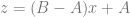
Remembering that the equation for a linear function is 


So, we start with the power series bilinear interpolation polynomial:
Which becomes this after substitution:

After some expansion and simplification we get this:

This formula tells us the value we get if we have a bilinear interpolation of values A,B,C,D (aka a bilinear surface defined by those points), and we sample along the x,y line defined by
It’s a very generalized function that’s hard to reason about much, but one thing is clear: it is a quadratic function! Whatever constant values you choose for A,B,C,D,m and b, you will get a quadratic polynomial (or lower degree, but never higher).
Here’s a shadertoy that shows curves generated by random sub pixel line segments on a random (white noise) RGB texture: https://www.shadertoy.com/view/XstBz7
(note that the rough edges of the curve are due to the fact that interpolation happens in X.8 fixed point format, so has pretty limited precision. Check the paper for more information and ways to address the issue.)

Let’s explore a bit by plugging in some values for 

m=0, b=0
Let’s see what happens when m is 0 and b is 0. In other words, lets see what happens when we sample along the line 
Plugging those values in gives:
interestingly, this is just a linear interpolation between A and B, which makes sense when looking at the graph of where we are sampling on the bilinear surface.

This goes along with what wikipedia told us: when one of the axes is constant (it’s a horizontal or vertical line) the result is linear.
m=1, b=0
Let’s try m = 1 and b = 0. That is the line: 

Plugging in the values gives us this equation:

We get a quadratic out! This shouldn’t be too surprising. This is the original insight in the technique. This is also the formula for a quadratic Bezier curve with control points 


m=2, b=1
Let’s try the line 

Plugging in the values give us the equation:

Once again we got a quadratic function when sampling along a line.
You might think it’s strange that the equation ends it “+C” instead of “+A”, but if you look at the graph it makes sense. The line literally starts at C when x is zero.
x=2u, y=3u
In the above examples we are only modifying the y variable, to be some function of x. What if we also want to modify the x variable?
One way to do this is to make a 3rd variable 

Let’s see what happens when we use these two equations:


That makes us sample this line on the bilinear surface.

Plugging the functions of u in for x and y we get:

It’s still a quadratic!
What About a Quadratic Path?
So we now know that when moving along a straight line on a bilinear surface, that you will get a quadratic function as output, except in the case of the line being horizontal or vertical. Note: if the bilinear surface is a plane, all lines on that surface will be linear functions, so this is another way to get a linear result. It could also be degenerate and give you a point result. You will never get a cubic result (or higher) when going along a straight line though.
What would happen though if instead of sampling along straight lines, we sampled on other shapes, like quadratic curves?
y=x*x
Let’s start with the function

Going back to the power series form of bilinear interpolation, let’s plug 
The starting equation:
becomes:

Which becomes:

It’s a cubic equation!
Here is a shadertoy which follows this sampling path on random pixels: https://www.shadertoy.com/view/4sdBz7

Something neat about this example specifically is that a cubic equation has 4 coefficients, which are basically 4 control points. This example makes use of the values of the 4 pixels involved to come up with the 4 coefficients, so “doesn’t leave anything on the table” so to speak.
This is unlike sampling along line segments where you have 3 control points stored in 4 pixel values. One is a bit redundant in that case.
You can make use of that fact (I have for instance!), but sampling along a quadratic path to get a cubic curve feels like a natural fit.
x=u*u, y=u*u
Let’s see what happens when we move along both x and y quadratically.
Just like in the linear case, we have our 3rd variable u that goes from 0 to 1 and we have x and y be based on that variable. We will use these equations:


The sampling path looks like this:

When we plug those in we get this quartic function:

You might be surprised to see what looks like a linear path. It’s just because at all times, x is the same value as y, even though they travel down the line non linearly.
Shadertoy: https://www.shadertoy.com/view/Xdtfz7

Higher Order Curves: x=3u^2, y=2u^4
Let’s get a little more wild, using these equations:


Which makes a sampling path of this:

Plugging in the equations, the bilinear interpolation equation:
becomes a hexic equation:

The shadertoy visualizes it on random pixels as per usual, but with u going from 0 to 1, it means that x goes from 0 to 3 (y is still 0-1), which makes some obvious discontinuities at the boundaries of pixels. In our pure math formulation, we wouldn’t have any of those, but since we are sampling a real texture, when we leave the safety of our (0,1) box, we enter a new box with different control points. https://www.shadertoy.com/view/4dtfz7

Trigonometric Function: y = sin(2*pi*x)
Let’s try 

The bilinear interpolation equation becomes a trigonometric polynomial:

That has disconuities in it when texture sampling again, due to leaving the original pixel region, so here’s a better looking shadertoy, which is for 

Circle
Lastly, here’s sampling on a circle.


It follows this path:

Plugging the functions into the power series bilinear equation gives:

Here’s the shadertoy: https://www.shadertoy.com/view/Xddfz7

Something neat about sampling in a circle is that it’s continuous – note how the left side of the curves line up with the right side seamlessly. That seems like a pretty useful property.
Moving On
We went off into the weeds a bit, but hopefully you can see how there are a ton of possibilities for encoding and decoding data in a very small number of pixels by carefully crafting the path you sample along.
Compared to the simple “sample along the diagonal” technique, there is some added complexity and shader instructions though. Namely, any work you do to modify x or y before passing them to the linear texture interpolator needs to happen in shader code. That means this technique takes more ALU, but can mean it takes even less texture memory than the other method.
The last question from the top of the post is “What does this all mean in higher dimensional interpolation, like trilinear or quadrilinear?”
Well, it works pretty much the same was as bilinear but there are more dimensions to work with.
We saw that in 2 dimensional bilinear interpolation that when we made x and y be functions (either of each other, or of a 3rd variable u), that the resulting polynomial had a degree that was the degree of x plus the degree of y.
In 3 dimensions with trilinear interpolation, the resulting polynomial would have a degree that is the degree of x, plus the degree of y, plus the degree of z.
In 4 dimensions with quadrilinear, add to that the degree of w.
Let’s consider the case when we don’t want a single curve though, but want a surface or (hyper) volume.
As we’ve seen in the extension dealing with surfaces and volumes, if you have a degree N polynomial, you can break it apart into a multivariate polynomial (aka a surface or hyper volume) so long as the sum of the degrees of each axis adds up to N.
It’s basically what we were just talking about but in reverse.
One thing I think would be interesting to explore further would be to see what the limitations are when you take this “too far”.
For instance, a 2×2 texture can give you a quadratic if you sample along any straight line in the uv coordinates. If you first put the u coordinate through a cubic function, and put the v coordinate through a different cubic function, I think you should be able to make a bicubic surface.
The surface will be constrained to a subset of what a general bicubic surface is able to be shaped like, but you will get a bicubic surface. (basically there will be implicit control points that you don’t have control over unless you add more pixels, and do more sampling, or higher dimensional linear interpolation)
I’d like to see what the constraints there are and see if there’s any chance of getting any real use out of something like that.
Anyhow, thanks for reading! Any ideas, corrections, usage cases you have, whatever, hit me up!

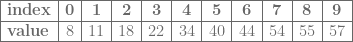

 is the sum of all the values in the rectangle from
  to
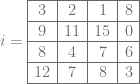
to  inclusively, but what if we want to find the sum of a different rectangle? What if we have 4 points A,B,C,D and we want to know the sum of the numbers within that sub-rectangle?


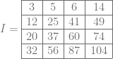
 more bits of storage which means we would need 2 more bits of storage in this case for the 2×2 grid (4 samples), making it be 5 bits total per value (3 bits of storage + 2 extra bits to hold the sum of 4 values). That would let us store the proper table:
 is 0.
is 0. is 2.
is 2.