Bezier Curves Part 2 (and Bezier Surfaces)

This is a follow up post to Bezier Curves. My plan was to write a post about b-splines and nurbs next, but after looking into them deeper, I found out they aren’t going to work for my needs so I’m scratching that.

Here’s some basic info on b-splines and nurbs though before diving deeper into Bezier curves and surfaces.

B-Splines (Basis Splines)

Bezier curves are nice, but the more control points you add, the more complex the math gets because the degree of the curve function increases with each control point added. You can put multiple Bezier curves end to end to be able to have more intricate curves, but another option is to use B-Splines.

B-Splines are basically Bezier curves which let you specify more control points without raising the degree of the Bezier curve. They do this by having control points only affect part of the total curve.

This way, you could make a quadratic b-spline which had 10 control points. Only a few control points control any given point on the curve, so the curve stays quadratic (and so does the math), but you get a lot more control points. A “Knot Vector” is what controls which parts of the curve the control points control.

A Bezier curve is actually a special case of B-Spline where all control points affect the entire curve.

Nurbs (Non Uniform Rational B-Spline)

Sometimes when working with curves, you want some control points to be stronger that others. You can accomplish this in Bezier curves and B-splines by doubling up or trippling up control points in the same location to make that control point twice, or three times as strong respectively.

What if you want a control point to be 1.3 times stronger though? That gets a lot more complicated.

Nurbs solve that problem by letting you specify a weight per control point.

Just like Bezier curves are a special case of B-Splines, B-Splines are a special case of nurbs. A B-Spline could be thought of as nurbs that has the same weighting for all control points.

Back to Bezier!

My end goal is to find a curve / surface type that is flexible enough to be used to make a variety of shapes by artists, but is efficient at doing line segment tests against on the GPU. To this end, B-Splines and Nurbs add algorithmic and mathematical complexity over Bezier curves, and seem to be out of the running unless I can’t find anything more promising.

My best bet right now looks like a Bezier Triangle. Specifically, a quadratic Bezier triangle, where each side of the triangle is a quadratic Bezier curve that has 3 control points. When I get those details fully worked out, I’ll report back, but for now, here’s some interesting info I found about generalizing bezier curves both in order (linear, quadratic, cubic, quartic, etc) as well as in the number of dimensions (line, curve, triangle, tetrahedron, etc).

Bezier Generalized

I found the generalized equation on the wikipedia page for Bezier triangles and am super glad i found it, it is very cool!

I want to show you some specifics to explain the generalization by example.
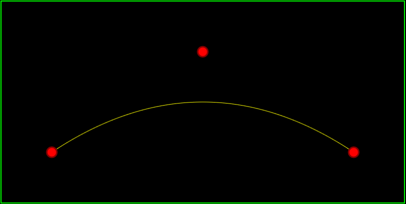
Quadratic Curve:
(A * S + B * T) ^ 2

Expanding that gives you:
A^2 * S^2 + A * B * 2 * S * T + B^2 * T^2

In the above, S and T are Barycentric Coordinates in a 1 dimensional Simplex. Since we know that barycentric coordinates always add up to 1, we can replace S with (1-T) to get the below:

A^2 * (1-T)^2 + A * B * 2 * (1-T) * T + B^2 * T^2

Now, ignoring T and the constants, and only looking at A and B, we have 3 forms: A^2, AB and B^2. Those are our 3 control points! Let’s replace them with A,B and C to get the below:

A * (1-T)^2 + B * 2 * (1-T) * T + C * T ^2

And there we go, there’s the quadratic Bezier curve formula seen in the previous post.
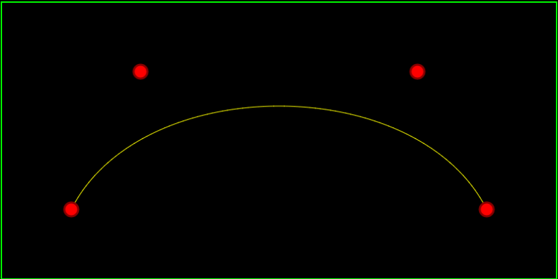
Cubic Curve:
(A * S + B * T) ^ 3

To make a cubic curve, you just change the power from 2 to 3, that’s all! If you expand that equation, you get:
A^3*S^3+3*A^2*B*S^2*T+3*A*B^2*S*T^2+B^3*T^3

We can swap S with (1-T) to get:

A^3*(1-T)^3+3*A^2*B*(1-T)^2*T+3*A*B^2*(1-T)*T^2+B^3*T^3

Looking at A/B terms we see that there is more this time: A^3, A^2B, AB^2 and B^3. Those are our 4 control points that we can replace with A,B,C,D to get:
A*(1-T)^3+3*B*(1-T)^2*T+3*C*(1-T)*T^2+D*T^3

There is the cubic Bezier curve equation from the previous chapter.

Linear Curve:
(A * S + B * T) ^ 1

To expand that, we just throw away the exponent. After we replace S with (1-T) we get:
A * (1-T) + B * T

That is the formula for linear interpolation between 2 points – which you could think of as the 2 control points of the curve.

One more example before we can generalize.

Quadratic Bezier Triangle:
(A * S + B * T + C * U) ^ 2

If you expand that you get this:
A^2*S^2+2*A*B*S*T+2*A*C*S*U+B^2*T^2+2*B*C*T*U+C^2*U^2

Looking at combinations of A,B & C you have: A^2, AB, AC, B^2, BC, C^2. Once again, these are your control points, and their names tell you where they lie on the triangle. A Bezier triangle is a triangle where the 3 sides of the triangle are bezier curves. A quadratic bezier triangle has quadratic bezier curves for it’s edges which mean that each side has 3 control points. Those 3 control points are made up of the 3 corners of the triangle, and then 3 more control points, each one being between end points. A^2, B^2 and C^2 represent the 3 corners of the triangle. AB is the third control point for the bezier curve on the edge AB. BC and AC follow that pattern as well! Super easy to remember.

In a cubic Bezier triangle, you get a lot more control points, but a new class of control point too: ABC. This control point is in the middle of the triangle like the name would imply.

Anyways, in the expanded quadratic bezier triangle equation above, when you replace the control points with A,B,C for the triangle corner control points (the squares) and D,E,F for the inbetween control points, you get the bezier triangle equation below:

A*S^2+2*D*S*T+2*E*S*U+B*T^2+2*F*T*U+C*U^2

Note that we are dealing with a simplex in 3d now, so once again, instead of needing ALL Barycentric coordinates (S,T,U) we could pick one and replace it. For instance, we could replace U with (1-S-T) to have one less variable floating around.

All Done for Now

You can use this pattern to expand either in “surface dimension”, or in the dimension of adding more control points (and increasing the order of the equation). I love it because it’s super simple to remember that simple equation, and then just re-calculate the equation you need for whatever your specific usage case is.

If this stuff is confusing, check out the wiki page for Bezier Triangles, it has a great graphic that really shows you what I’m trying to explain:
Bezier Triangle

Next up I either want to make an HTML5 interactive app for messing around with Bezier triangles, or if I can figure out how to intersect a line segment with a quadratic Bezier triangle, i’ll probably just have some real cool looking screenshots to post along w/ the equation I ended up using (;

Special thanks to wolfram alpha for crunching some of these equations. Check it out, it’s really cool!
Wolfram Alpha – Cubic Bezier Curve Expansion

For more bezier fun check out my next Bezier post: One Dimensional Bezier Curves.

Implicit vs Parametric vs Explicit Surfaces

Implicit Surface

It’s always R = 0 where R is a function of one or more variables.

Like the unit circle equation:
x^2 + y^2 -1 = 0.

Parametric Surface

The components of the output are based on some parameter or parameters

Like the quadratic bezier curve (which A,B,C and CurvePoint are points in N dimensions):
CurvePoint = f(t) = A*(1-t)^2 + B*2t(1-t) + C*t^2

Or the unit circle:
x = cos(t)
y = sin(t)

Or surfaces like this:
SurfacePoint3D = f(u,v)

Explicit Surface

The more usual looking type functions where you have one variable on the left side (dependent variable), and another variable on the right side (independent variable).

Like lines:
y = mx + b

or height fields:
height = f(x,y)

More Info

Here’s a cool set of slides that explain this stuff in more detail (and beyond), and the pros and cons of using various forms.

Representing Smooth Surfaces

Bezier Surface Properties

Here’s a couple pretty cool properties of Bezier surfaces that I learned recently.

The first one is that if you consider a “convex hull” being made up of the control points (connect all the control points into a convex shape), the curve will lie entirely inside that shape. That means you can use the shape of the control points as a “quick test” for rendering or collision detection. Note though, you could also just make a sphere that enclosed all the control points and do a sphere test instead, if you would rather have a simpler/quicker test at the cost of some wasted space (more false positives).

The second interesting property is that you can do back face culling of a Bezier surface if all the control points face away from the camera. while it’s true this isn’t EXACTLY proper back face culling, the odds are good it’s good enough for your needs, especially given how quick a test it is.

The third interesting property is that if you want to transform a bezier surface with something like a translation, rotation, or scale, you can apply the transform to the control points, and the curve will be transformed by the same transformation.”A Bézier surface will transform in the same way as its control points under all linear transformations and translations.” (from Wikipedia: Bezier Surface)

… but unfortunately, as promising as these properties are, it still seems infeasible to render a decent number of bezier surfaces via real time raytracing (something i was planning on) and it seems to only get worse when moving to b-splines and nurbs surfaces, so it seems like this may not be the way to go. It’s still possible though that raymarching these surfaces could be doable, but I haven’t explored too much in that direction yet.

Bezier Curves

Bezier curves are pretty cool. They were invented in the 1950s by Pierre Bezier while he was working at the car company Renault. He created them as a succinct way of describing curves mathematically that could be shared easily with other people, or programmed into machines to make curves that matched the ones created by human designers.

I’m only going to go over bezier curves at the very high level, and give some links to html5 demos I’ve made to let you play around with them and understand how they work, so you too can implement them easily in your own software.

If you want more detailed information, I strongly recommend this book: Focus on Curves and Surfaces

Quadratic Bezier Curves

Quadratic bezier curves have 3 control points. The first control point is where the curve begins, the second control point is a true control point to influence the curve, and the third control point is where the curve ends. Click the image below to be taken to my quadratic bezier curve demo.


bezquad

A quadratic bezier curve has the following parameters:

  • t – the “time” parameter, this parameter goes from 0 to 1 to get the points of the curve.
  • A – the first control point, which is also where the curve begins.
  • B – the second control point.
  • C – the third control point, which is also where the curve ends.

To calculate a point on the curve given those parameters, you just sum up the result of these 3 functions:

  1. A * (1-t)^2
  2. B * 2t(1-t)
  3. C * t^2

In otherwords, the equation looks like this:

CurvePoint = A*(1-t)^2 + B*2t(1-t) + C*t^2

To make an entire curve, you would start with t=0 to get the starting point, t=1 to get the end point, and a bunch of values in between to get the points on the curve itself.

Cubic Bezier Curves

Cubic bezier curves have 4 control points. The first control point is where the curve begins, the second and third control points are true control point to influence the curve, and the fourth control point is where the curve ends. Click the image below to be taken to my cubic bezier curve demo.


bezcubic

A cubic bezier curve has the following parameters:

  • t – the “time” parameter, this parameter goes from 0 to 1 to get the points of the curve.
  • A – the first control point, which is also where the curve begins.
  • B – the second control point.
  • C – the second control point.
  • D – the fourth control point, which is also where the curve ends.

To calculate a point on the curve given those parameters, you just sum up the result of these 4 functions:

  1. A * (1-t)^3
  2. B * 3t(1-t)^2
  3. C * 3t^2(1-t)
  4. D * t^3

In otherwords, the equation looks like this:

CurvePoint = A*(1-t)^3 + B*3t(1-t)^2 + C*3t^2(1-t) + D*t^3

Math

You might think the math behind these curves has to be pretty complex and non intuitive but that is not the case at all – seriously! The curves are based entirely on linear interpolation.

Here are 2 ways you may have seen linear interpolation before.

  1. value = min + percent * (max – min)
  2. value = percent * max + (1 – percent) * min

We are going to use the 2nd form and replace “percent” with “t” but they have the same meaning.

Ok so considering quadratic bezier curves, we have 3 control points: A, B and C.

The formula for linearly interpolating between point A and B is this:
point = t * B + (1-t) * A

The formula for linearly interpolating between point B and C is this:
point = t * C + (1-t) * B

Now, here’s where the magic comes in. What’s the formula for interpolating between the AB formula and the BC formulas above? Well, let’s use the AB formula as min, and the BC formula as max. If you plug the formulas into the linear interpolation formula you get this:

point = t * (t * C + (1-t) * B) + (1-t) * (t * B + (1-t) * A)

if you expand that and simplify it you will end up with this equation:
point = A*(1-t)^2 + B*2t(1-t) + C*t^2

which as you may remember is the formula for a quadratic bezier curve. There you have it… a quadratic bezier curve is just a linear interpolation between 2 other linear interpolations.

Cubic bezier curves work in a similar way, there is just a 4th point to deal with.

Next Up

The demos above are in 2d, but you could easily move to 3d (or higher dimensions!) and use the same equations. Also, there are higher order bezier curves (more control points), but as you add control points, the computational complexity increases, so people usually stick to quadratic or cubic bezier curves, and just string them together. When you put curves end to end like that, they call it a spline.

Next up, be on the look out for posts and demos for b-splines and nurbs!