The C++ code that goes with this post can be found at https://github.com/Atrix256/AlgorithmX

A fun youtube video came out recently showing how people optimized an algorithm from running for an entire month, to eventually running for less than a millisecond: https://www.youtube.com/watch?v=c33AZBnRHks

In that video, algorithm X was mentioned and I was intrigued. Giving it a google, I found this 2018 video by Knuth talking about his “Algorithm X” method to solve exact cover problems, specifically using “Dancing Links” to implement it efficiently: https://www.youtube.com/watch?v=_cR9zDlvP88

So what is an exact cover problem? If you have some tetrominoes (or Tetris pieces) and you want to put them together to form a rectangle, that is an exact cover problem. If you want to put N queens on an NxN chess board such that none can attack each other, that is an exact cover problem. Solving sudoku is also an exact cover problem.

A more formal definition is on Wikipedia at https://en.wikipedia.org/wiki/Exact_cover. Interestingly it says that you can turn any NP problem into an exact cover problem!

I wanted to learn this algorithm to have something in my tool belt to approach these sorts of problems more intelligently, but I also think this will lead to new algorithms for generating noise textures (aka sampling matrices), and/or new types of situationally optimal noise.

Let’s talk about the details of the algorithms a bit and then look at some examples.

Exact Cover Problems

An exact cover problem is described by a binary matrix of 0s and 1s.

Using Knuth’s terminology, the columns are called items and are the things that are looking to be covered. For example, for placing objects on a chess board, there would be an item (matrix column) per chess board location.

Rows are called options and they contain one or more items that they cover. For example, a tetromino at a specific position on a chess board would cover multiple chess board locations. That option (matrix row) would have a 1 at each of those locations and a 0 at the rest of the locations.

The goal of an exact cover problem is to find a set of options which cover all items exactly once.

An extension to this idea is to have some items be optional. These items don’t have to be covered, but if they are covered, they can only be covered at most once. We’ll make use of this in the N-Queens example.

There are other extensions that I’ll briefly explain at the bottom of this post.

Algorithm X

Knuth’s Algorithm X is a method for solving exact cover problems. At the highest level, it works like this.

1. Choose an item to cover from the list of items. (only choose from required items)
2. For each option that covers that item, try it as part of the solution:
   • Remove each item that option covers. All those items can be considered covered.
   • Remove all options that have items that were removed. They are no longer valid choices since they conflict.
   • Recurse, having Algorithm X solve the problem with reduced items.
   • Undo making this option part of the solution and try the next option.

If the item list becomes empty (or only has optional items left), you have a valid solution.

If any item runs out of valid options, you’ve hit a dead end.

Depending on the problem you are trying to solve, you may find 0 solutions, 1 solution, or multiple solutions. If you are only looking for one solution instead of all possible solutions, you can exit out after finding a solution.

Note that even though you iterate through all the options that cover an item in step 2, you don’t need to iterate through the items in step 1. Recursing will choose the other items, and you will reach all possible solutions.

In step 1 you can choose an item to cover however you want. A very good way to do it though is to choose the item with the fewest items left which is also “the hardest item to cover”. That is what Knuth recommends, and from observation, it aggressively culls the search tree without changing the solutions that can be reached, so is great stuff. In the IGN example, i’ll talk about how this was the difference between a 24 minute run of the algorithm, and a less than 1 millisecond run of the algorithm for the same exact cover problem!

As far as the order that options are tried in, Knuth recommends either doing them in order, or in a randomized order.

In the code I made for this post, if you only want one solution, it will visit the options in random order, but if you want all options, it will do them in order and save the cost of gathering up and shuffling the options.

Dancing Links

Dancing links is a technique that can be used when implementing Algorithm X to efficiently add and remove items and options.

One observation in Algorithm X is that the matrix is usually pretty sparse with a lot of 0s. Usually, an individual option only covers a few items, and the vast majority of items are left uncovered by that option.

To deal with this, you can make a doubly linked list of items within an option, only putting in the items that are covered.

Having a sparse matrix made up of doubly linked lists makes it easy to remove nodes, by just doing this:

node->left->right = node->right;
node->right->left = node->left;
node->left = nullptr;
node->right = nullptr;

An observation about doubly linked lists is that you can remove a node from a list but leave the node’s pointers in tact. You do the first 2 lines above but not the bottom 2 lines. If you do that, you can put this node back into the list by just doing this:

node->left->right = node;
node->right->left = node;

This allows you to undo any number of node removals, so long as you re-insert them in the reverse order that you removed them. This reverse order handling comes naturally in a recursive algorithm, such as Algorithm X.

Using doubly linked lists for a sparse matrix, and leaving removed nodes “dirty” to be able to quickly undo their removal are the core concepts of using dancing links to implement Algorithm X. This allows items and options to be removed and restored very efficiently, allowing Algorithm X to be very, very fast.

Implementation Details

Knuth’s code implements the linked lists as using integer indices into an array, instead of pointers, with the reasoning that they can be smaller than a pointer (like in x64, a 32 bit int is half size) and so are more cache friendly. Another nice thing about using integer indices is that they don’t become invalid if you resize a dynamic array, which I use (Knuth uses fixed size arrays).

I have a list of items, where an item looks like this:

// An item is something to be covered
struct Item
{
    char name[8];
    int leftItemIndex = -1;
    int rightItemIndex = -1;
    int optionCount = -1;
};

The name is a label describing the item and is only useful for user friendliness. If you removed it, the algorithm would still work and it would probably be more cache friendly.

There is also an extra item on the end of the list that serves as the “root node” of the linked list. This is the node you start from when iterating through the items.

An “itemIndex” is the index that an item occurs in the m_items array. The left and right item index are the previous and next items in the available items list.

The “optionCount” is a count of how many items there are available for an item. This helps the item with the lowest count be found more quickly when deciding which item to cover next.

The other data type is a node:

// An option is a sequential list of nodes.
struct Node
{
    // Spacer nodes use upNodeIndex as the index of the previous spacer node, and downNodeIndex as the next spacer node.
    // Non spacer nodes use these to get to the next option for the current item
    int upNodeIndex = -1;
    int downNodeIndex = -1;

    // What item a node belongs to.
    // -1 means it is a spacer node.
    // There is a spacer node before and after every option.
    // An option is a sequential list of nodes.
    int itemIndex = -1;
};

Each item has a node, and in fact, the itemIndex is also the index into the m_nodes array where the node lives for that item.

The upNodeIndex and downNodeIndex goes up and down in the sparse array, so starting at the node of an item and iterating through that list is how you find the options available for that item.

Options also have nodes. They have one node per item in the option, and are laid out sequentially in the m_nodes array so that you can add one to a node index to go to the next item in the option, or subtract one from the node index to go to the last item in the option. The itemIndex of a node is the item that the node belongs to.

There is also a “spacer node” at the beginning of each option which can be identified by having an itemIndex of -1. In this case, the upNodeIndex is the previous spacer node, and the downNodeIndex is the next spacer node. This is useful when iterating through all items in an option to be able to go back to the beginning of the option. There is also a spacer node at the end of the options to simplify code by being able to make the assumption that there is always a spacer node at the beginning and end of the items.

The other thing worth mentioning is that when covering an item, you remove it from the list of items, and then have all current options of that item remove themselves from all other lists except the item being covered. This is necessary so that when this item is uncovered, you can iterate through the options that it still knows about, and have each add itself back into the necessary lists (restore the up and down pointers).

With the implementation details out of the way, let’s see this algorithm in action!

Basic Examples

The code for this section is in BasicExamples() in main.cpp.

Knuth has a basic example in his write up (https://www-cs-faculty.stanford.edu/~knuth/programs/dlx1.w):

The items are A,B,C,D,E,F,G where F and G are optional.

The options are:

• CEF
• ADG
• BCF
• AD
• BG
• DEG

The goal is to find the set of options which covers A,B,C,D,E and optionally may cover F or G, but if they do, must only cover it once.

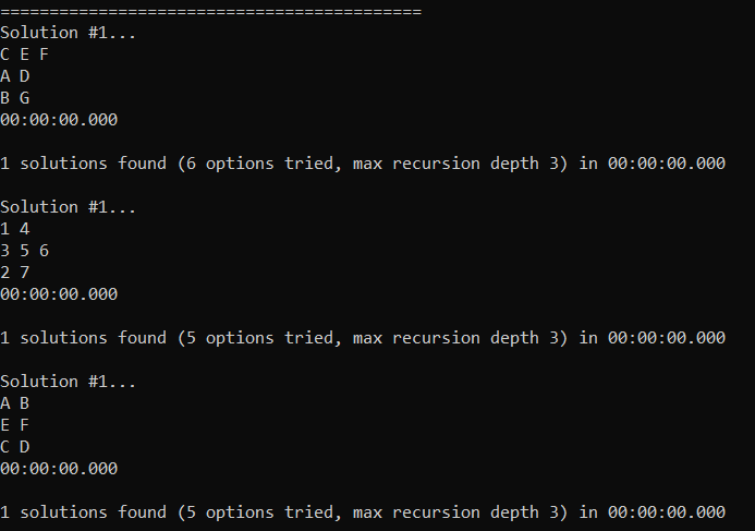
Running the code that goes with this blog post agrees with what he says the right answer is…

There is only one solution, which is to use the options: CEF, AD, BG

Wikipedia has another simple example (https://en.wikipedia.org/wiki/Exact_cover#Detailed_example):

The items are 1,2,3,4,5,6,7 and they are all required.

The options are:

• 147 (named A)
• 14 (named B)
• 457 (named C)
• 356 (named D)
• 2367 (named E)
• 27 (named F)

Once again there is only a single solution, which is 14 (B), 356 (D), 27 (F).

Wikipedia then goes on to talk about an “Exact Hitting Set” (https://en.wikipedia.org/wiki/Exact_cover#Exact_hitting_set) which is different than an exact cover problem, but is solved by transposing the exact cover matrix and then solving that. Check the wikipedia page for a description of what sort of problems these are.

The items to cover are the names of the options: A, B, C, D, E, F.

Since the matrix is transposed from the exact cover problem, each option (row) is the list of options in the previous problem which contain each number 1 through 7:

• AB (these are the ones that contained a 1 in the last problem)
• EF (ditto for 2)
• DE (3)
• ABC (4)
• CD (5)
• DE (6)
• ACEF (7)

Solving that gives a single answer again: AB, EF, CD.

These are basically diagnostic tests to help make sure the algorithm is working, and help show how it works.

Here is the program output. It found the solutions amazingly fast (< 1 millisecond), but that isn’t too surprising as these are pretty simple problems.

N-Rooks

Now for something a little more tangible… let’s say we had a standard 8×8 chess board and we are trying to place 8 rooks on it such that no rook could attack any other rook.

The code for this section is in NRooks.h.

In this problem, each row must have a rook in it (and only 1), so we have 8 required items named Y1 through Y8. Each column must also have a rook in it (and only 1), so we have 8 more required items named X1 through X8 making for 16 items total.

You then make an option for each location on chess board, which means 64 options total.

Within each option, you put a 1 for the row and column that is covered by placing a rook there. Putting a 1 in an item for an option means just having that item be in the list for that option.

For instance, placing a rook at location (0,0) on the chess board would put a 1 in X0 and a 1 Y0. Placing a rook at location (4,5) would put a 1 in X4 and a 1 in Y5.

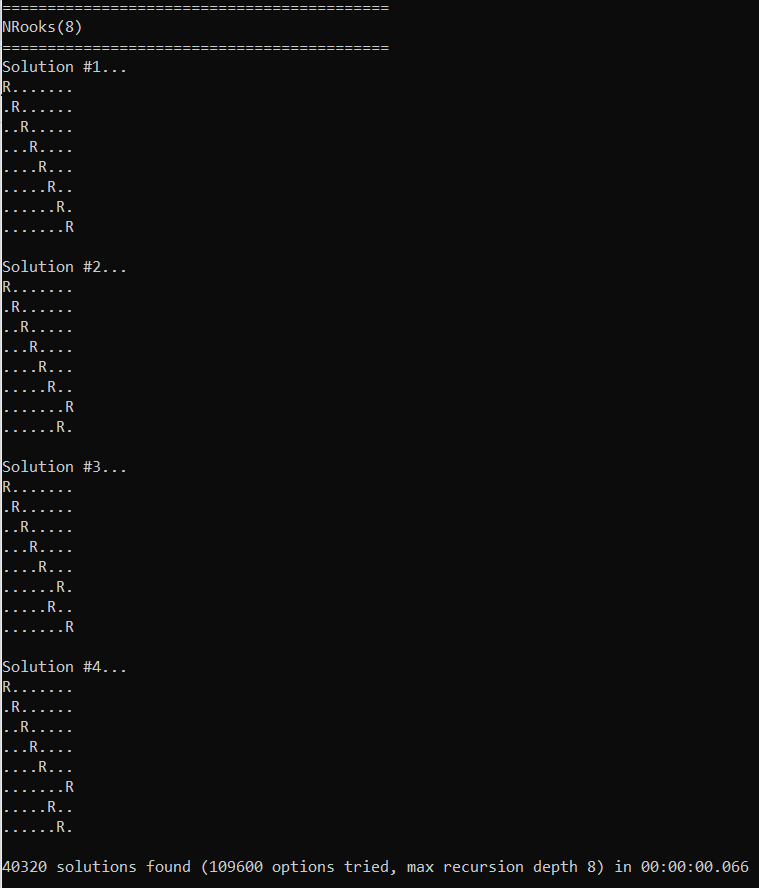
Below is the program output, where it found 40320 solutions in 66 milliseconds, and shows the first 4 solutions it found.

This is for a standard 8×8 chess board with 8 rooks on it, but the problem (and supplied code!) generalizes to an NxN chess board with N rooks on it and is called the N-Rooks problem.

N-Queens

The N-Queens problem is the same as the N-Rooks problem, but using queens instead of rooks.

The code for this section is in NQueens.h.

We use the same items for queens as we do for rooks, but we also add the diagonals since queens can attack diagonally. In this case, there are more than N diagonals though so we can’t require that all diagonals are used by queens. We deal with this by making the diagonals be optional items.

There are 2N-1 diagonals going left, and 2N-1 diagonals going right, so for when N=8, we add 30 optional items to the 16 required items that rooks have.

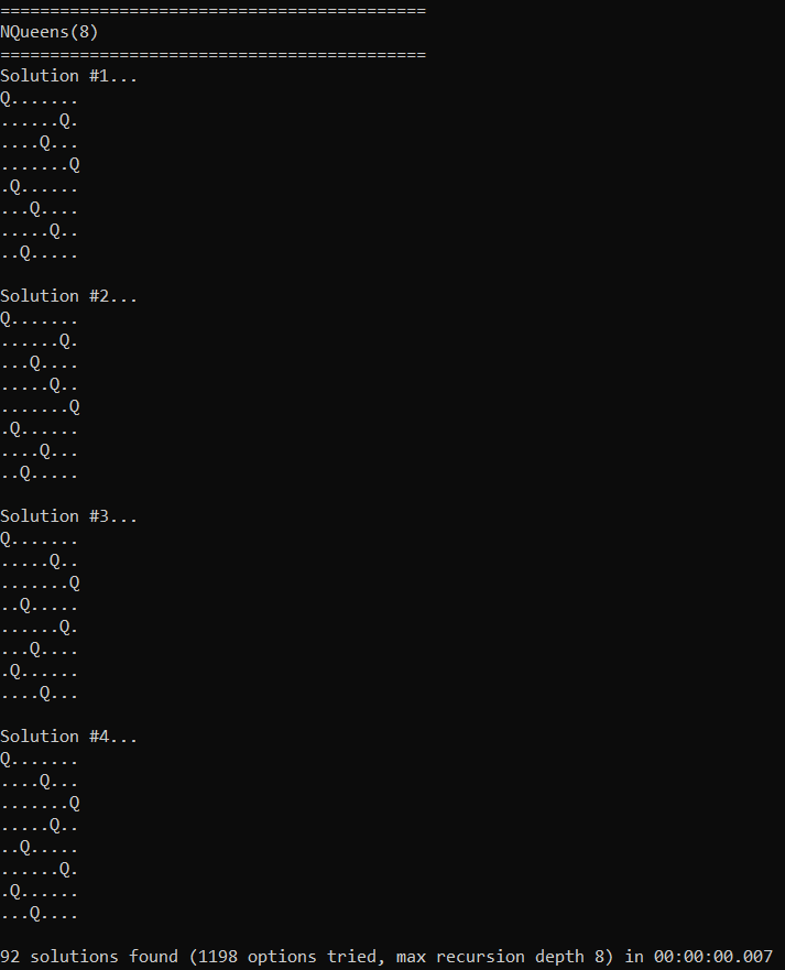
The results are below… 92 solutions found in 7 milliseconds! Wikipedia agrees that there are 92 solutions https://en.wikipedia.org/wiki/Eight_queens_puzzle.

For comparison, when N=12 it finds all answers in 600 ms. When N=13 it finds them in 2.7 seconds. When N=14 it finds them (365,596 solutions) in 14 seconds. Don’t forget that this is a single threaded algorithm running on the CPU!

Sudoku

The code for this section is in Sudoku.h.

Sudoku is a game played on a 9×9 grid where there are some numbers 1-9 already present on the board and you need to fill in the blank spots such that each row has all numbers 1-9 exactly once, so does each column, and so does each 3×3 block of cells (9 total 3×3 blocks of cells, they don’t overlap).

For solving sudoku, the items to cover are all required and they are:

• 81 for cells: Each of the 81 cells must have a value (it doesn’t matter which value)
• 81 for columns: Each of the 9 columns must have each possible value 1-9.
• 81 for rows: Each of the 9 rows must have each possible value 1-9.
• 81 for blocks: Each of the nine 3×3 blocks must have each possible value 1-9.
• 1 for initial state: Since there is an initial state for the board, one option will describe the initial state and this item ensures that it is always part of any solution found.

That makes for a total of 325 items to cover.

As far as options go, there will be one option for each value in each cell, which means 81*9 = 729 options. We only make options for the cells where the initial state is blank though, which cuts down the actual number of options needed. In our example, we’ll have 30 numbers already covered, leaving 51 uncovered. That means we’ll only need 51*9 = 459 options.

There will also be one option for the initial state, which is the only one that has the initial state item covered, making for a total of 460 options.

As an example of what an option looks like, let’s consider the option of putting a 4 in (3,5). That option will have the following items:

• Cell (3,5) has a value in it
• Column 3 has a 4 in it.
• Row 5 has a 4 in it.
• Block (1,2) has a 4 in it.

Each option has to describe all the things it covers.

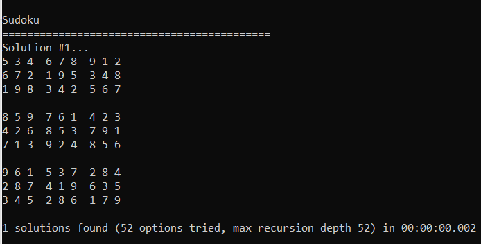
Wikipedia has an example Sudoku problem that I plugged in (https://en.wikipedia.org/wiki/Sudoku) and then ran the program. It was able to find the same solution listed on wikipedia and verify that it only had one solution, in 2 milliseconds.

Plus Noise

The code for this section is in PlusNoise.h.

I have a blog post that talks about a “Plus Noise Low Discrepancy Grid” (https://blog.demofox.org/2022/02/01/two-low-discrepancy-grids-plus-shaped-sampling-ldg-and-r2-ldg/). This is a 5×5 matrix of numbers where if you look at any pixel, and the 4 cardinal direction neighbors (toroidally wrapping around at the edges) that it will have each number 1 through 5.

The post shows how to find a formula for that grid, but let’s try see what this algorithm can come up with.

Our items to cover will be:

• 25 for cells: Each of the entries in the 5×5 matrix needs to have a value (but it doesn’t matter what value is there).
• 125 for plus shapes: There is a plus shape with a center point of each entry in the matrix, so 25 plus shapes. Each plus shape needs each value 1 through 5, so 25*5 = 125 items.

That makes for 150 items total.

As far as options, we need an option for each possible value at each possible location, which means 25*5 = 150 options.

As an example, the option for putting a 2 in (3,4) would have these items:

• Cell (3,4) has a number
• The plus with a center at (3,4) has a 2 in it.
• The plus with a center at (2,4) has a 2 in it. (The plus to the left)
• The plus with a center at (4,4) has a 2 in it. (The plus to the right)
• The plus with a center at (3,3) has a 2 in it. (The plus above)
• The plus with a center at (3,0) has a 2 in it. (The plus below. Note the y axis wraps here)

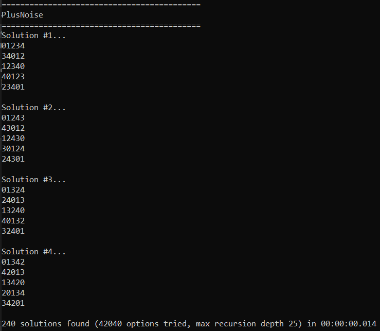
Running that finds 240 solutions in 14 milliseconds! The original blog post found the formula (x+3y)%5, but after looking at the results, I realized that (x+2y)%5 is also a solution. So that takes care of 2 solutions, what about the other 238?

Well, one thing to realize is that if you have a solution, you can swap any 2 numbers and have another valid solution. This means that you essentially have 5 symbols (0,1,2,3,4) that you can arrange in any way to find a different solution. That means 5! = 120 solutions. Since there are two different formulas for generating this 5×5 matrix, and each has 120 solutions, that accounts for the 240 solutions this found.

Something interesting is that I tried this with smaller (3×3 and 4×4) grid sizes and it wasn’t able to find a solution. Trying larger sized grids, I was only able to find solutions when the size was a multiple of 5, and it still would only find 240 solutions. This matrix tiles, so this all makes a decent amount of sense. The larger sizes that are multiples of 5 just found a solution by tiling the 5×5 solution, interestingly.

Interleaved Gradient Noise (IGN)

The code for this section is in IGN.h.

In a previous blog post I wrote about Interleaved Gradient Noise, which is a low discrepancy grid created by Jorge Jimenez while he was at Activision (https://blog.demofox.org/2022/01/01/interleaved-gradient-noise-a-different-kind-of-low-discrepancy-sequence/). IGN is a screen space noise designed to leverage the neighborhood sampling that temporal anti aliasing uses to know when to keep or reject history. Using IGN as the source of per pixel random numbers in stochastic rendering under TAA thus gives better renders for the same costs. It works even better than blue noise in this situation, believe it or not.

This noise is a generalized sudoku where the rows and columns must all have values 1 through 9, but instead of only the 9 main 3×3 blocks needing to have each value 1 through 9, it’s EVERY 3×3 block needing to have that, including overlapping blocks. There is a block with a center at each location of the 9×9 matrix, so there are 81 3×3 blocks.

The items are then…

• 81 for cells: Each of the 81 cells must have a value (it doesn’t matter which value)
• 81 for columns: Each of the 9 columns must have each possible value 1-9.
• 81 for rows: Each of the 9 rows must have each possible value 1-9.
• 729 for blocks: Each cell is the center of a 3×3 block, and each of them must have each value 1-9. So 81*9 = 729 items.

This is 891 items to cover.

Note there is no initial state in this setup, unlike the sudoku section. We want it to find ANY solution it can.

The number of options is still that each cell could have each possible value, so its 81*9 = 729 options.

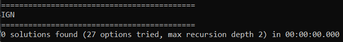
It rapidly found that there were no solutions. It took less than a millisecond and the search space ended up being very small. Having the program spit out the steps it was taking (look for SHOW_ALL_ATTEMPTS), I found that it was able to quickly find a situation that couldn’t be satisfied and that it was right.

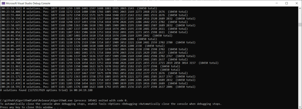
Fun fact, I previously had it choosing items to cover from left to right, instead of covering the item with the fewest options remaining. When I did that, the program took 25 minutes to find the answer as you can see below! The cover fewest options item heuristic is pretty powerful, and gives some intuition behind why the Wave Function Collapse algorithm (https://github.com/mxgmn/WaveFunctionCollapse) has the same heuristic – collapse whichever item has the fewest options.

So this algorithm confirms that there is no exact solution to the constraints that IGN sets up. IGN is an approximate solution though, and has numerical drift across space to distribute the error of not exactly solving the constraints. IGN itself was tuned by hand and eye, so I would bet is not be the optimal formula for being an approximate solution to these constraints. I’m not sure how you’d find the optimal formula though (let’s say, optimal in a least squared error sense?).

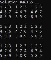
Anyhow it made me think… as far as TAA is concerned, it’s primarily the 3×3 block constraints that matter to the neighborhood sampling, and not the rows and columns constraints. So, I made an IGNRelaxed() function which doesn’t have them. After running for 13 minutes, it’s found 49,536 solutions. I don’t have a very exact way to measure progress but it didn’t seem anywhere near done so I killed it.

I’m not sure if this sampling pattern would be any good in practice. On one hand, it is optimized towards TAA’s neighborhood sampling, but it doesn’t have anything to fight regular structure or promote diversity of values in small regions. Maybe it has a use, maybe not. If you give it a try, let me know!

UPDATE: Extensions Briefly Explained

Here are some other extensions to this algorithm:

• Knuth’s DLX2 has the ability for optional items to have a color, and be allowed to be covered by any number of items of the same color. An example usage case is in making a cross word puzzle. The letters could be the color, and it’s ok if two words claim the same letter in the same cell where the words overlap.
• DLX3 allows you to specify a min and max number of coverings per item instead of requiring exactly 1 coverings. This could let you set up constraints like putting N queens and 1 king on a chess board and making it so between 2 and 4 of the queens must be attacking the king.
• DLX5 lets you give a cost per option, and a tax (discount) per item. This lets you find minimum cost solutions. The cost doesn’t drive the search though, unfortunately. It searches exhaustively and gives you the k best scoring solutions.

I’ll bet you can imagine other extensions as well. This basic algorithm seems very natural to modify towards other specific goals, or constraint types.

Closing & Links

AlgorithmX using Dancing Links is super powerful and super fast. I feel like more folks need to know about these techniques.

My goal was to see if this algorithm (+ extensions) could be used as an alternative to void and cluster and simulated annealing for generating noise textures (sampling matrices). After learning more, it looks like it could, but only in narrow & rare usage cases. It has the ability to score solutions, but the scoring doesn’t drive the search. For making blue noise without any other hard constraints, it would just be a brute force search then.

I think this algorithm could be made multithreaded if needed, by splitting the “search tree” up and giving a piece to each thread. It’s hard to know how to split this fairly though, so might need some sort of work stealing setup. I’m not real sure, but it seems doable.

Links:

Knuth’s talk about this topic: https://www.youtube.com/watch?v=_cR9zDlvP88

Knuth’s writeup on AlgorithmX and Dancing Links (DLX1): https://www-cs-faculty.stanford.edu/~knuth/programs/dlx1.w

Here are other programs he has written, including extensions to DLX (DLX2, DLX3, etc): https://www-cs-faculty.stanford.edu/~knuth/programs.html

Wikipedia:

• Algorithm X: https://en.wikipedia.org/wiki/Knuth%27s_Algorithm_X
• Dancing Links: https://en.wikipedia.org/wiki/Dancing_Links
• Exact Cover: https://en.wikipedia.org/wiki/Exact_cover

The video that started me down this rabbit hole: https://www.youtube.com/watch?v=c33AZBnRHks

@kmett (https://twitter.com/kmett) did a live coding youtube video of this algorithm: https://www.youtube.com/watch?v=IoXDNWhN0aw

Here is his explanation of it too: https://twitter.com/kmett/status/1585133038135975936?s=20&t=0IWdGtwBR-vN1V26eIN68A