I’ve heard that when sampling in 1D, such as ![x \in [0,1]](https://s0.wp.com/latex.php?latex=x+%5Cin+%5B0%2C1%5D&bg=ffffff&fg=666666&s=0&c=20201002)
![[0,1]^2](https://s0.wp.com/latex.php?latex=%5B0%2C1%5D%5E2&bg=ffffff&fg=666666&s=0&c=20201002)
That came up in a recent conversation (https://mastodon.gamedev.place/@jkaniarz/110032776950329500), so this post looks at the evidence of whether or not that is true – looking at regular sampling, blue noise sampling, and low discrepancy sequences (LDS). LDS are a bit of a tangent, but it’s good to see how they converge in relation to the other sampling types.
To be honest, my interest in blue noise has long drifted away from blue noise sample points and is more about blue noise textures (and beyond! Look for more on that soon), but we’ll still look at blue noise in this post since that is part of what the linked conversation is about!
I’ve lost interest in blue noise sample points because they aren’t very good for convergence (although projective blue noise is interesting https://resources.mpi-inf.mpg.de/ProjectiveBlueNoise/ProjectiveBlueNoise.pdf), and they aren’t good at making render noise look better. Blue noise textures are better for the second but aren’t the best for convergence (even when extended temporally), so they are mainly useful for low sample counts. This is why they are a perfect match for real-time rendering.
The value remaining in blue noise sample points in my opinion, are getting them as the result of a binary rendering algorithm, such as stochastic transparency. There the goal isn’t really to generate them though, but more that you want your real time algorithm’s noise to roughly follow their pattern. Blue noise sample points have value in these situations for non real time rendering too, such as stippling.
Anyhow, onto the post!
The code that goes with this post is at https://github.com/Atrix256/SampleAwayFromEdges
It turns out there is a utility to generate and test sample points that since you are reading this post, you may be interested in: https://github.com/utk-team/utk
1D Numberline Sampling
This group of tests will primarily look at two types of 1D sampling: regular sampling and blue noise sampling. The golden ratio low discrepancy sequence, stratified sampling and white noise are also included.
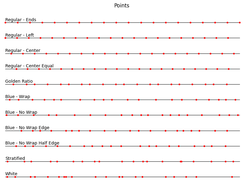
So first up, let’s talk about the different regular sampling options. The difference between these all is how you calculate the position of sample 


- Regular Ends:
. 4 samples would be at 0/3, 1/3, 2/3 and 3/3.
- Regular Left:
. 4 samples would be at 0/4, 1/4, 2/4 and 3/4.
- Regular Center:
. 4 samples would be at 1/8, 3/8, 5/8, 7/8.
- Regular Center Equal:
. 4 samples would be at 1/5, 2/5, 3/5, 4/5.
Believe it or not, which of those you choose has a big difference for the error of your sampling!
There are also four flavors of blue noise.
- Blue Wrap: Blue noise is made on a 1D number line using Mitchell’s Best Candidate algorithm, using wrap-around distance. A point at 1.0 is the same as a point at 0.0.
- Blue No Wrap: Same as above, but distance does not wrap around. A point at 1.0 is the farthest a point can be from 0.0.
- Blue No Wrap Edge: Same as above, but the algorithm pretends there are points at 0.0 and 1.0 that repel candidates by including the distance to the edge in their score.
- Blue No Wrap Half Edge: Same as above, but the distance to the edge is divided by 2, making the edge repulsion half as strong.
Lastly, there is also:
- White Noise: white noise random numbers that go wherever they want, without regard to other points.
- Stratified: This is like “Regular Left” but a random number
is added in.
.
- Golden Ratio: This is the 1D golden ratio low discrepancy sequence.
.
Here are 20 of each:
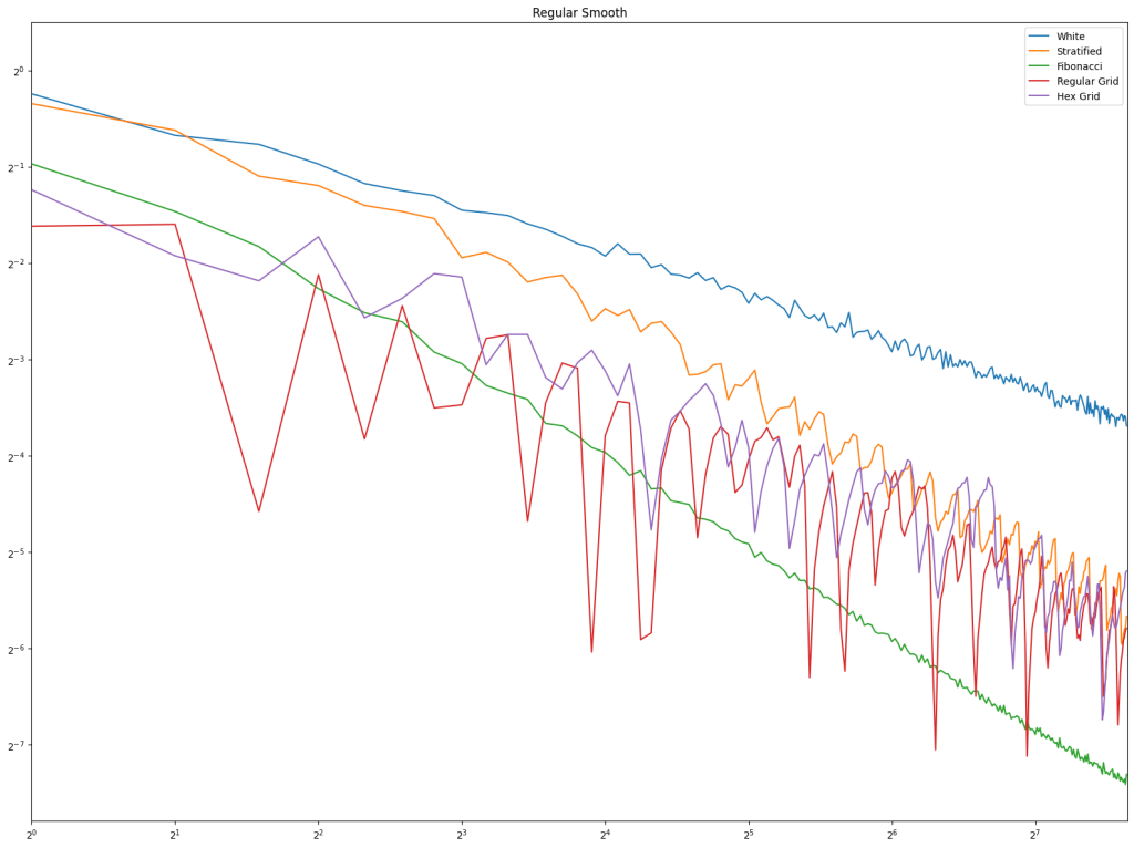
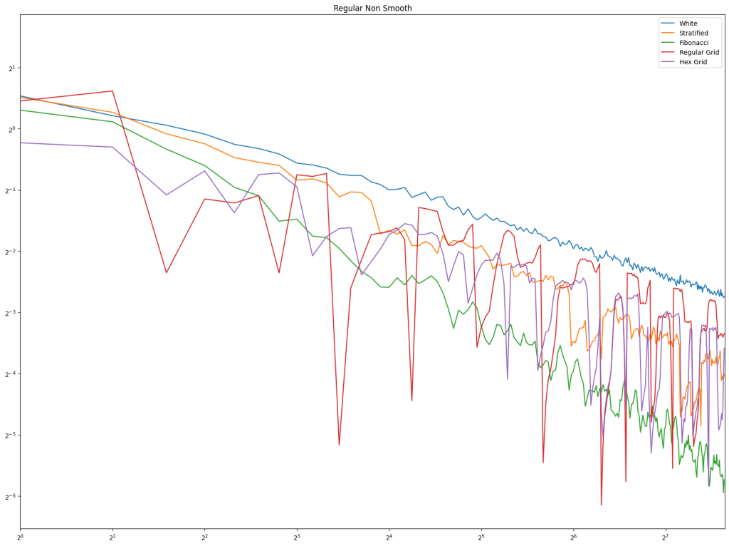
Those sequences are tested on both smooth and non-smooth functions:
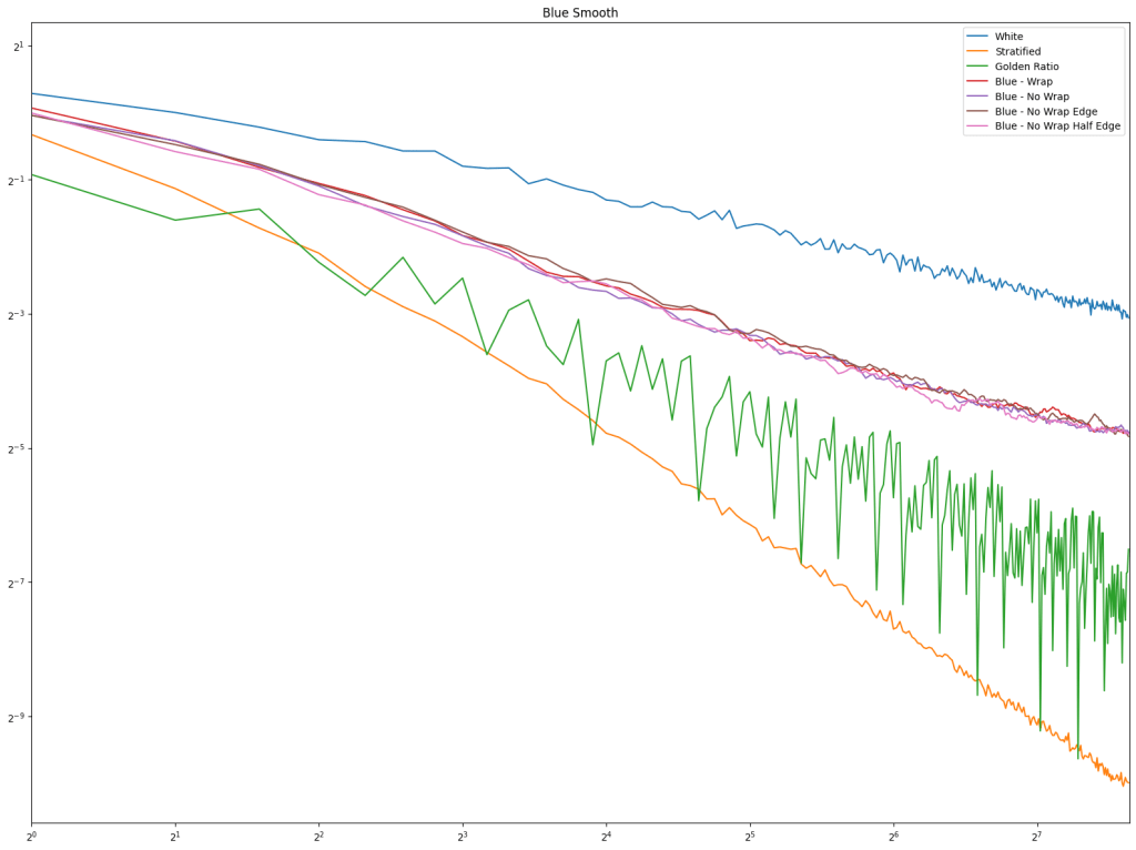
- Smooth: A cubic Bezier curve is randomly generated with each of the four control points between -10 and 10, and each sequence is used to integrate the curve using 200 points. This is done 1000 times to calculate RMSE graphs.
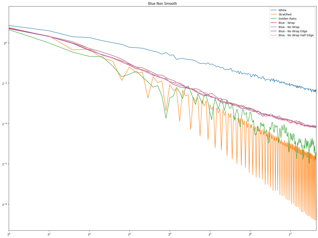
- Non Smooth: A random line is generated for each of the four 1/4 sized regions between 0 and 1. The two end points of the line are generated to be between -10 and 10, so the lines are usually not
continuous.
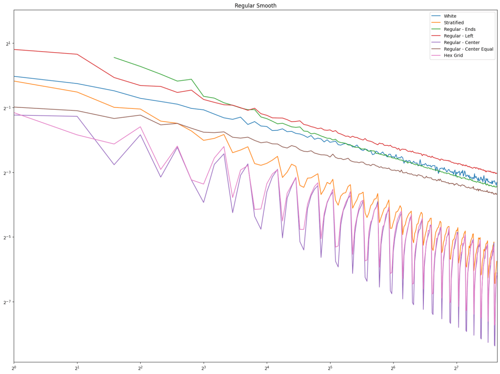
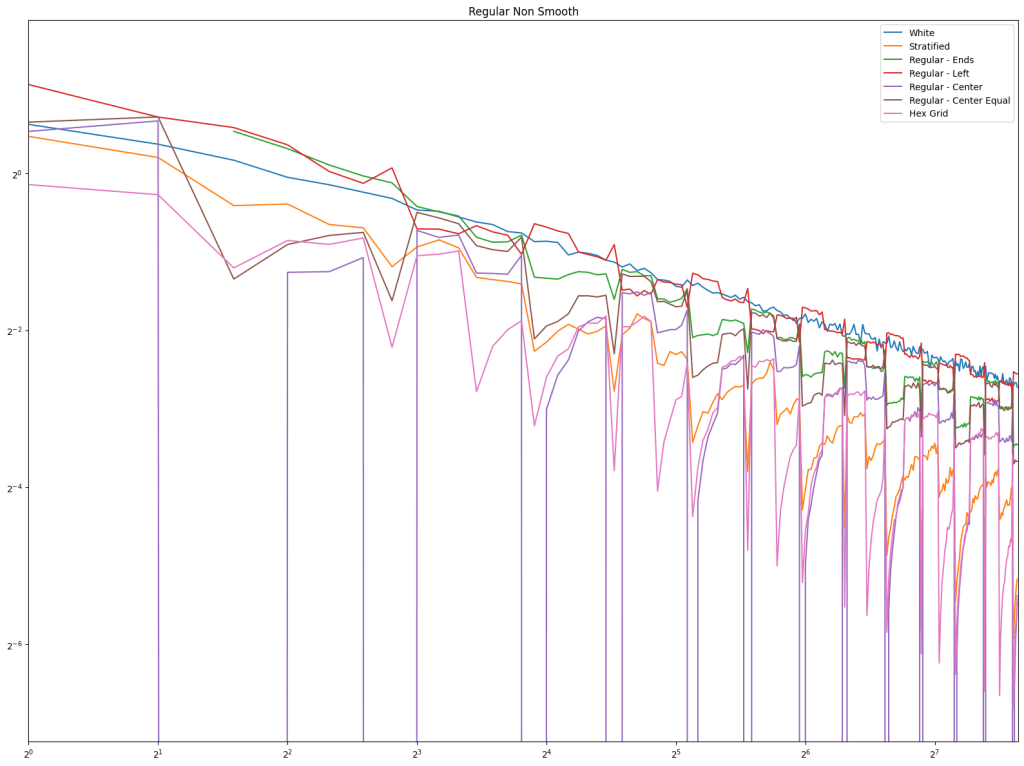
First let’s look at regular sampling of smooth and non smooth functions.
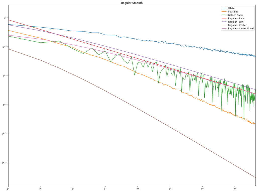
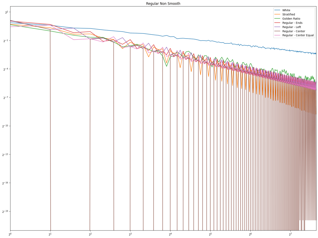
In both cases, white noise does absolutely terribly. Friends don’t let friends use white noise!
Also in both cases, the winner is “Regular Center” doing the best, with stratified sampling coming in second.
It’s important to note that while this type of regular sampling shows better convergence than stratified sampling, regular sampling has problems with aliasing that randomized sampling, like stratified, doesn’t have.
Looking at blue noise sampling next, it doesn’t seem to really matter whether you wrap or not. White noise, stratified, and golden ratio are included to help compare blue noise sampling with the regular sampling types.
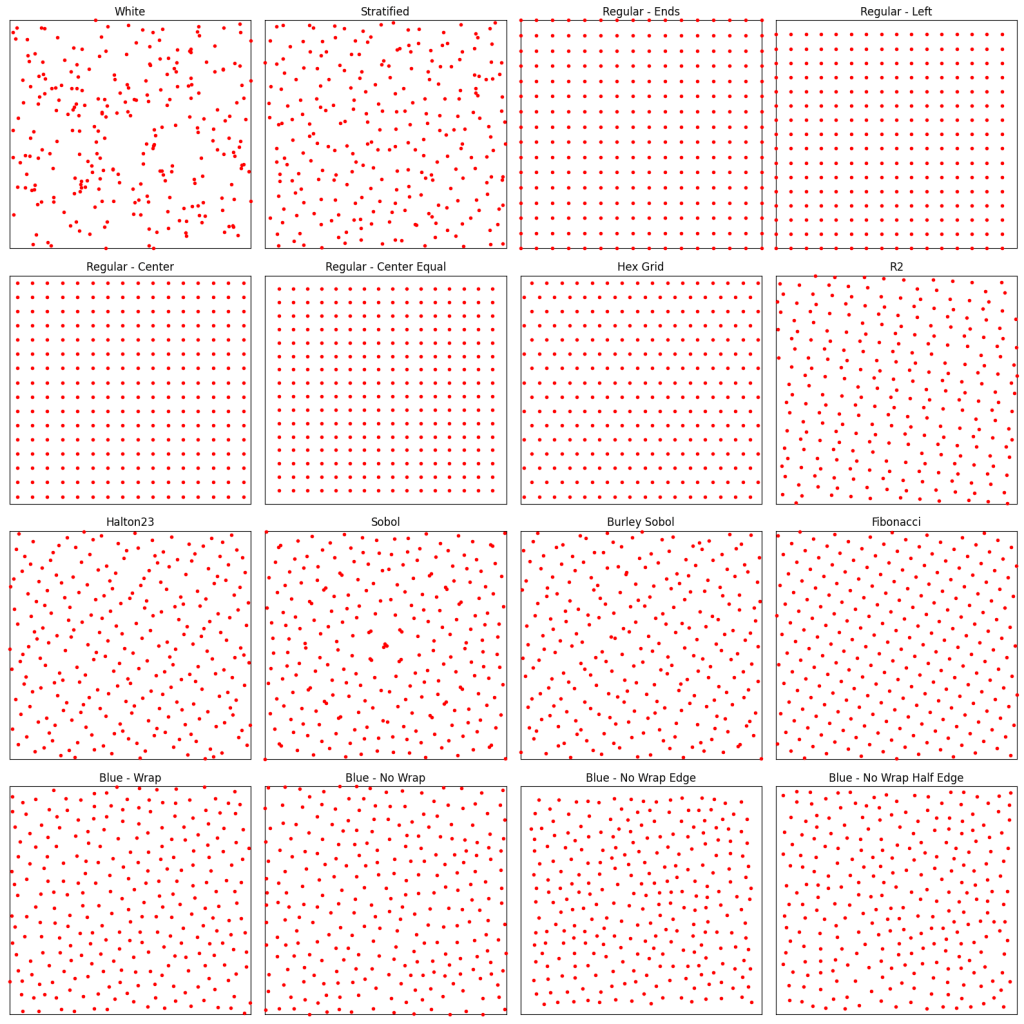
2D Square Sampling
The sampling types used here are:
- White Noise
- Stratified
- Regular Ends
- Regular Left
- Regular Center
- Regular Center Equal
- Hex Grid: Like regular grid, but each row is half a cell offset from the row above it.
- R2: The R2 sequence from Martin Roberts http://extremelearning.com.au/unreasonable-effectiveness-of-quasirandom-sequences/
- Halton(2,3)
- Sobol
- Burley Sobol: A scrambled sobol, from https://jcgt.org/published/0009/04/01/
- Fibonacci: The x axis is the golden ratio LDS, and the y axis is
- Blue Wrap
- Blue No Wrap
- Blue No Wrap Edge
- Blue No Wrap Half Edge

Here are 200 of each:
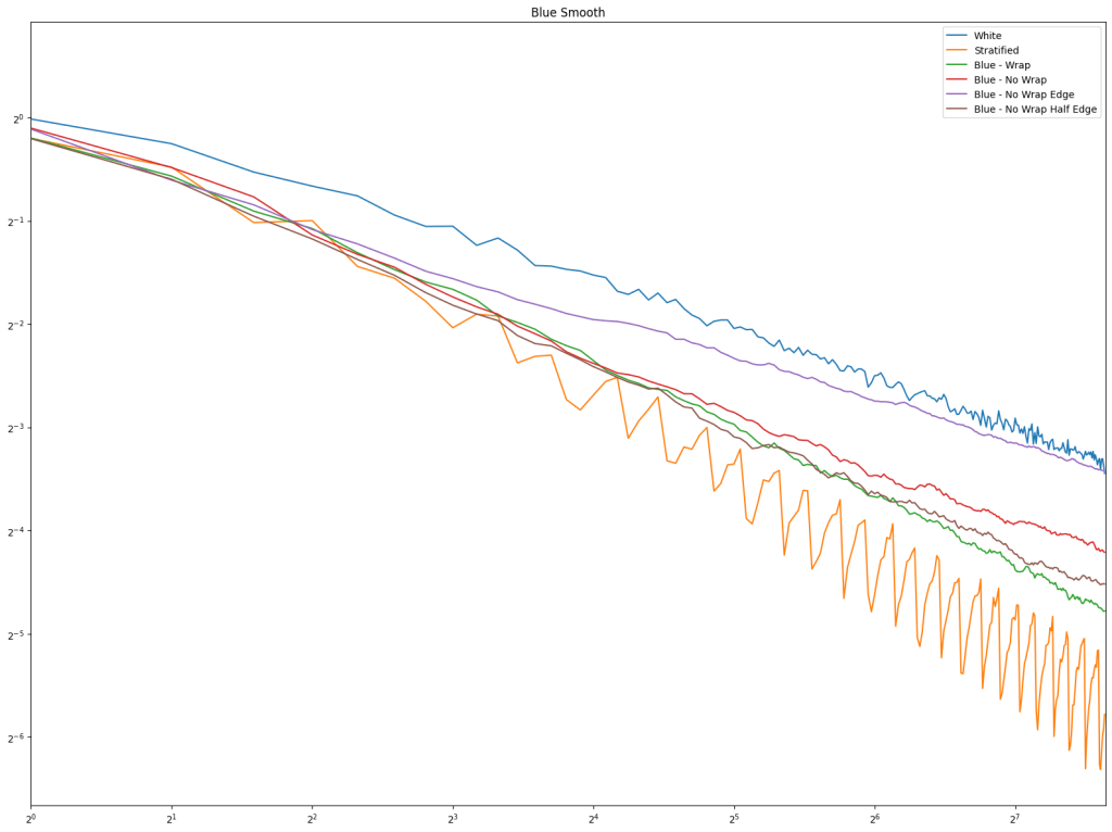
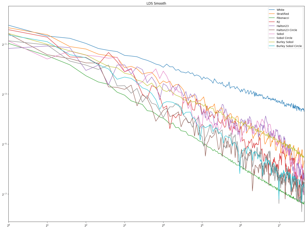
For the smooth tests, we generate a random bicubic surface, which has a grid of 4×4 control points, each being between -10 and 10.
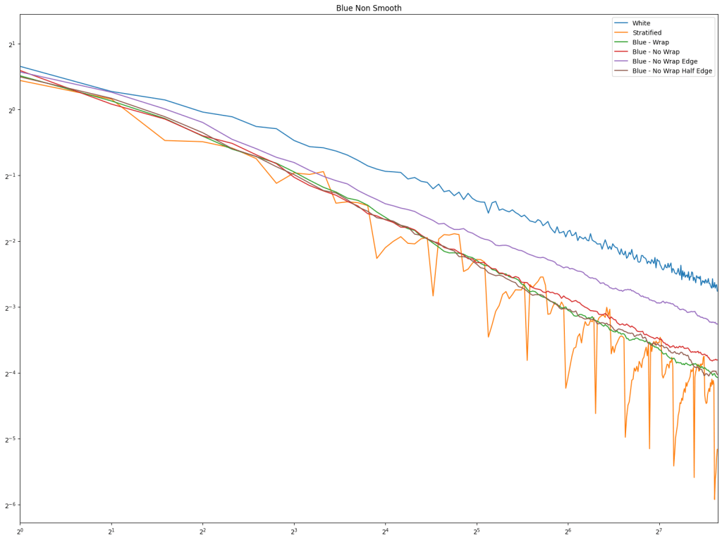
For the non smooth tests, we generate a 2×2 grid where each cell is a bilinear surface with 4 control points, so is not C0 continuous at the edges.
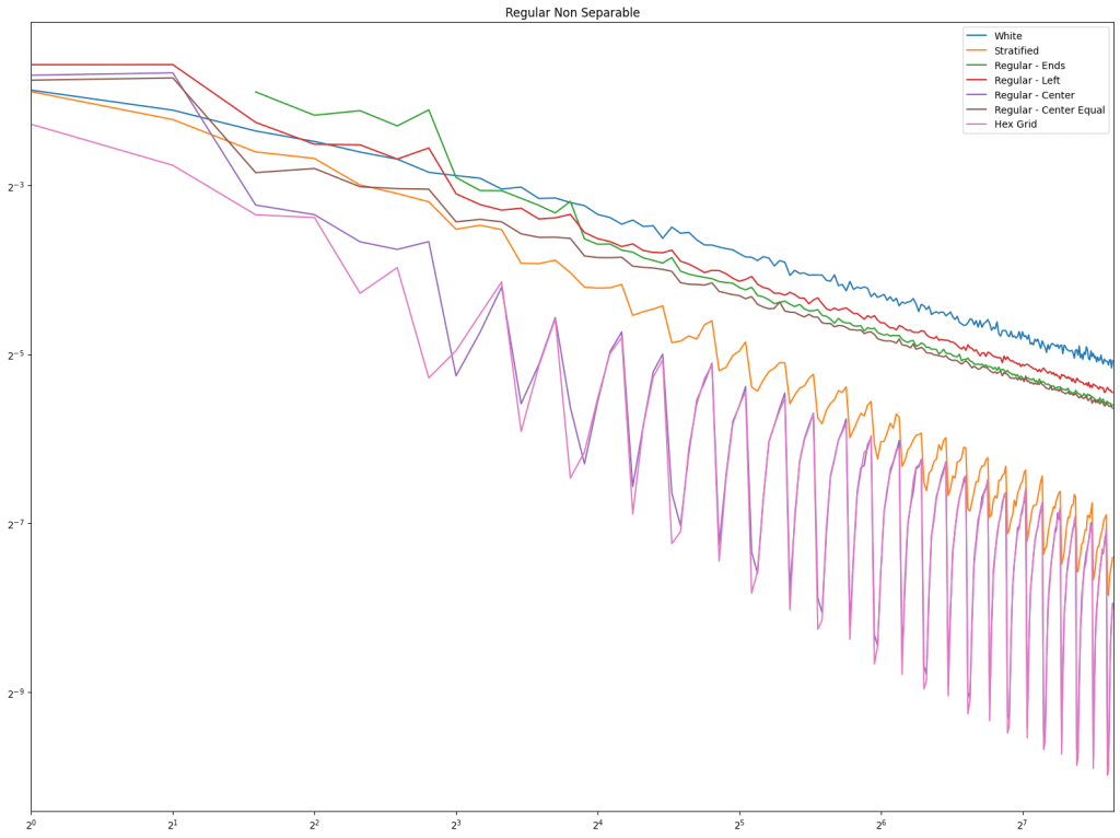
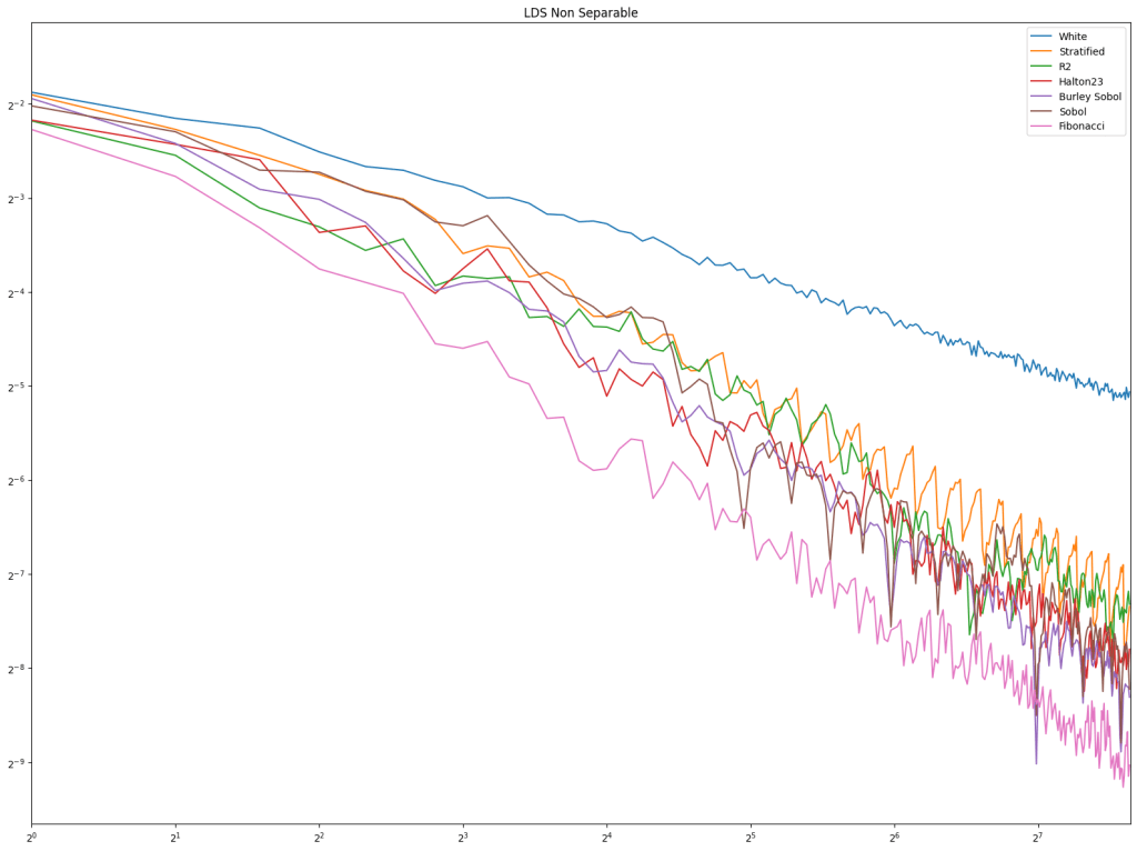
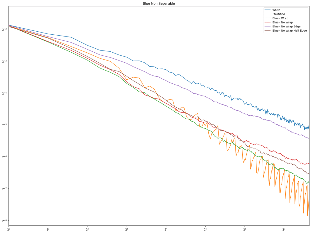
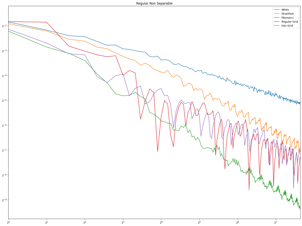
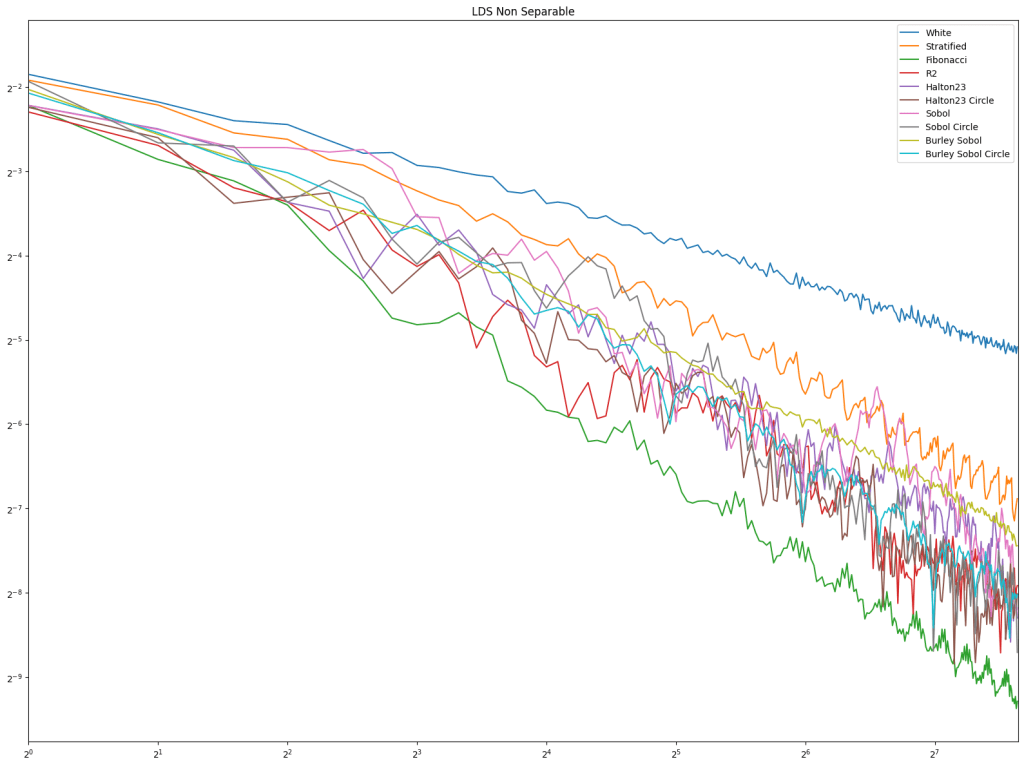
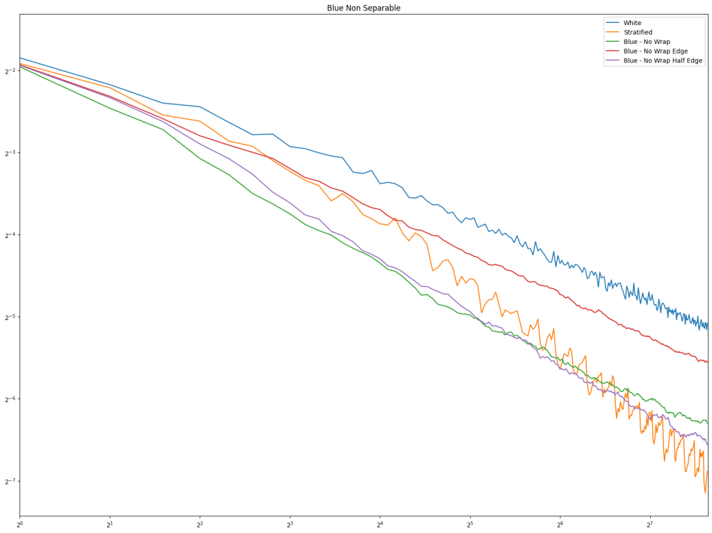
We also have a third test this time, for a function that is non separable. For this, we pick a random point as a grid origin, and a grid scale, and the value at each point in the square is the sine of the distance to the origin.
We once again do 1000 tests, with 200 samples per test.
First is regular sampling. White noise does terribly as always. Regular center is the winner, along with hex grid coming in second, and stratified in third. This shows that in 2D, like in 1D, avoiding the edges of the sampling domain by half a sample distance is a good idea.
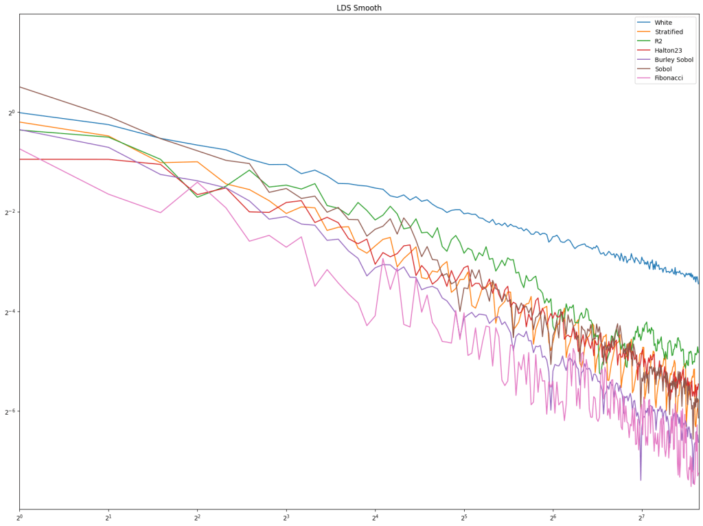
Next up is low discrepancy sequences. Fibonacci does well pretty consistently, but Burley Sobol also does. R2 doesn’t do very well in these tests, but these types of tests usually have much higher sample counts, and R2 is much more competitive there in my experience.

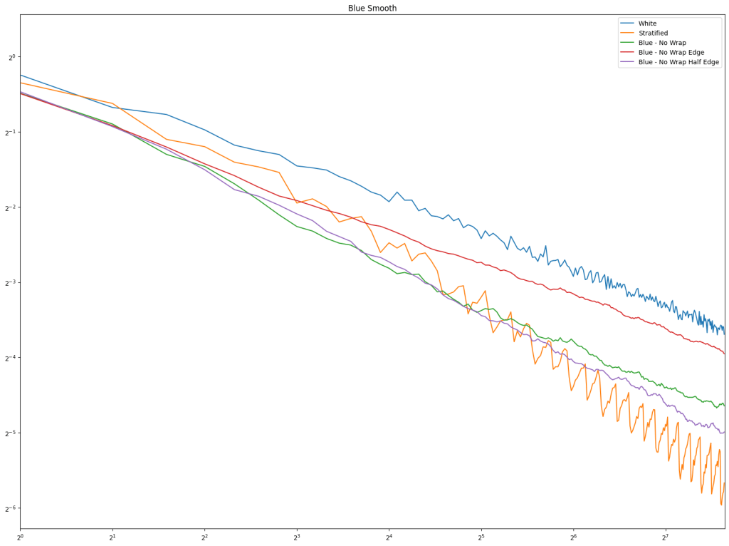
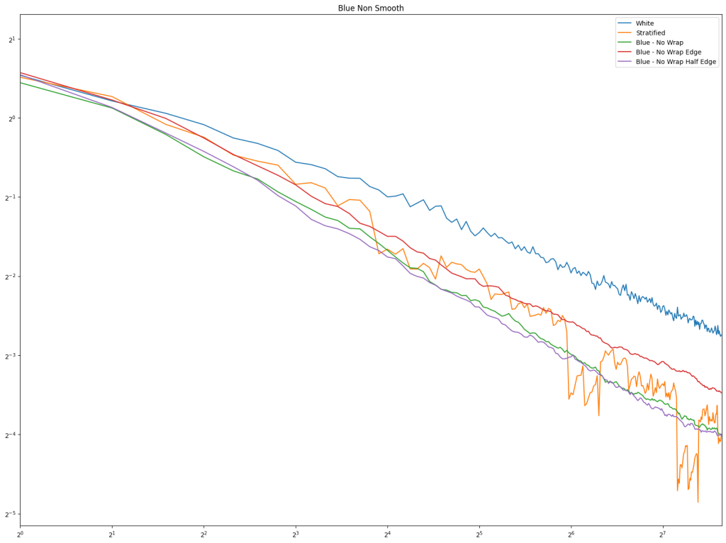
Lastly is the blue noise. Unlike in 1D, it does seem that blue noise cares about wrapping here in 2D, and that wrapping is best, with the half edge no wrapping being in second place. The half edge doing well also indicates that sampling away from the edges is a good idea. Blue noise sample points still don’t converge very well though.
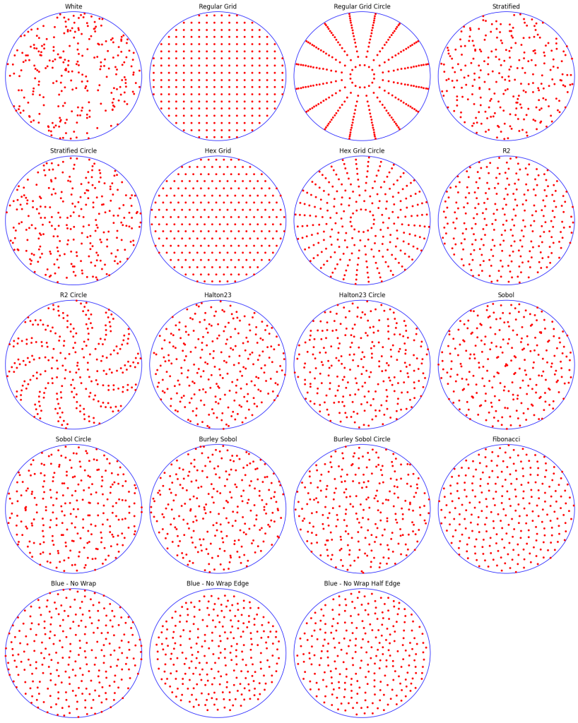
2D Circle Sampling
This last group of tests is on samples in a circle. Unlike a 1D numberline or a 2D square, there is no clear way to calculate “wrap around” distance. You might consider all points near the edge to be near each other, but that is one of many ways to think about wrap around distance in a circle. You could also consider all points near the edge to be next to the center of the circle perhaps.
The sampling used here is:
- White
- Regular Grid: “Regular center”, but points outside of the circle are rejected. This is done iteratively with more points until the right number of points fit in the circle. Since it can’t always exactly match the count needed, it gets as close as it can, and then adds white noise points to fill in the rest.
- Regular Grid Circle: “Regular center”, but x axis is multiplied by
to make an angle, and y axis is square rooted to make a radius. This transformation maps a uniform random point in a square to a uniform random point in a circle and will be used by other sampling types too.
- Stratified: angle and radius as stratified.
- Stratified Circle: A stratified square is mapped to circle.
- Hex Grid: With rejection and filling in with white noise.
- Hex Grid Circle: Hex grid is mapped to circle
- R2: with rejection
- R2 Circle: R2 mapped to circle.
- Halton23: with rejection
- Halton23 Circle: mapped to circle
- Sobol: rejection
- Sobol Circle: mapped to circle
- Burley Sobol: rejection
- Burley Sobol Circle: mapped to circle
- Fibonacci: mapped to circle
- Blue No Wrap
- Blue No Wrap Edge
- Blue No Wrap Half Edge
The tests are the same as 2D square, but the functions are zero outside of a radius 0.5 circle.
Here are 256 samples of each.
Looking at regular sampling first. Fibonacci dominates but the regular sampling beats stratified.
Looking at LDS next, fibonacci does pretty well in a class by itself, except for the non smooth test where burley sobol joins it.

Lastly is blue noise which seems to indicate that wrapping would be good, by “half edge” distance doing the best for the most part. This is also showing that sampling away from the edges is a good thing.
Conclusion
Looking at sampling a 1D number line, a 2D square, and a 2D circle, regular sampling and blue noise have shown that avoiding the edge of the sampling domain by “half a point distance” (repel at half strength for blue noise) gives best results.
It makes me wonder though: why?
If you have any thoughts, hit me up on:
- Twitter: https://twitter.com/Atrix256
- Mastodon: https://mastodon.gamedev.place/@demofox
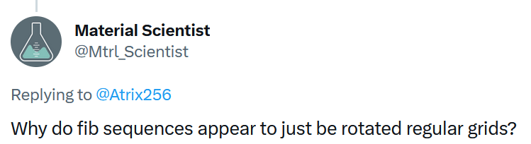
Fibonacci Looks Like a Rotated Grid, What Gives?
I got a good question on twitter after this post (https://twitter.com/Mtrl_Scientist/status/1644749290705649664?t=4MqnsDOpCSOwkfgvCqLXRw)
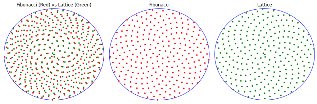
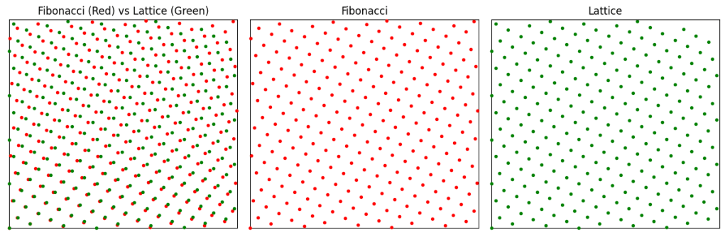
I don’t have much to say about why it looks like a rotated regular grid, but I can show how it’s different than one.
To do this, I grabbed 3 points of Fibonacci in a triangle, to get two vectors to use for lattice axes. I then used that to make a lattice that you can see below. Side by side Fibonacci and the lattice are hard to tell apart, but when they are put on top of each other, you can see how Fibonacci is not a lattice, but deviates from the lattice over space.
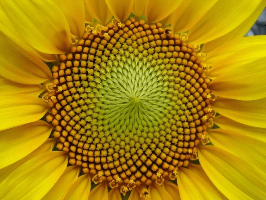
When we map it to a circle, the difference is more pronounced. The Fibonacci circle has that familiar look that you see in sunflowers. The Lattice however just looks like spirals. When they are overlaid, you can see they diverge quite a bit.