One Dimensional Bezier Curves

I was recently looking at the formula for bezier curves:

Quadratic Bezier curve:
A * (1-T)^2 + B * 2 * (1-T) * T + C * T ^2

Cubic Bezier curve:
A*(1-T)^3+3*B*(1-T)^2*T+3*C*(1-T)*T^2+D*T^3

(more info available at Bezier Curves Part 2 (and Bezier Surfaces))

And I wondered… since you can have a Bezier curve in any dimension, what would happen if you made the control points (A,B,C,D) scalar? In other words, what would happen if you made bezier curves 1 dimensional?

Well it turns out something pretty interesting happens. If you replace T with x, you end up with f(x) functions, like the below:

Quadratic Bezier curve:
y = A * (1-x)^2 + B * 2 * (1-x) * x + C * x ^2

Cubic Bezier curve:
y = A*(1-x)^3+3*B*(1-x)^2*x+3*C*(1-x)*x^2+D*x^3

What makes that so interesting is that most math operations you may want to do on a bezier curve are a lot easier using y=f(x), instead of the parameterized formula Point = F(S,T).

For instance, try to calculate where a line segment intersects with a parameterized bezier curve, and then try it again with a quadratic equation. Or, try calculating the indefinite integral of the parameterized curve so that you can find the area underneath it (like, for Analytic Fog Density). Or, try to even find the given Y location that the curve has for a specific X value. These things are pretty difficult with a parameterized function, but a lot easier with the y=f(x) style function.

This ease of use does come at a price though. Specifically, you can’t move control points freely, you can only move them up and down and cannot move them left and right. If you are ok with that trade off, these 1 dimensional curves can be pretty powerful.

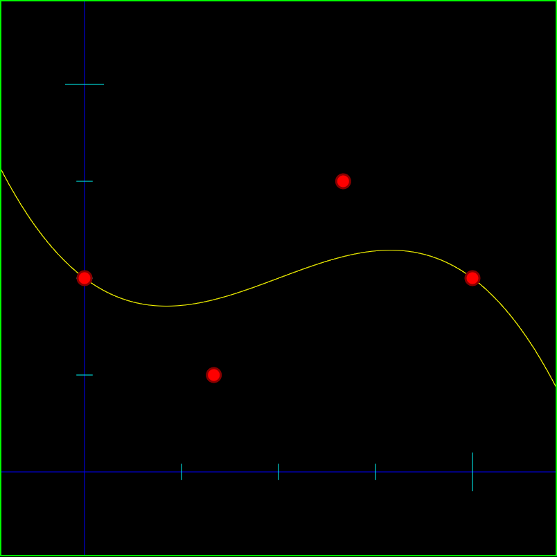
Below is an image of a 1 dimensional cubic bezier curve that has control points A = 0.5 B = 0.25 C = 0.75 D = 0.5. The function of this curve is y = 0.5 * (1-x)^3 + 0.25 * 3x(1-x)^2 + 0.75 * 3x^2(1-x) + 0.5 * x^3.

You can ask google to graph that for you to see that it is in fact the same: Google: graph y = 0.5 * (1-x)^3 + 0.25 * 3x(1-x)^2 + 0.75 * 3x^2(1-x) + 0.5 * x^3

cubicbez

Another benefit to these one dimensional bezier curves is that you could kind of use them as a “curve fitting” method. If you have some data that you wanted to approximate with a quadratic function, you could adjust the control points of a one dimensional quadratic Bezier curve to match your data set. If you need more control points to get a better aproximation of the data, you can just increase the degree of the bezier curve (check this out for more info on how to do that: Bezier Curves Part 2 (and Bezier Surfaces)).

Smoothstep as a Cubic 1d Bezier Curve

BIG THANKS to CeeJay.dk for telling me about this, this is pretty rad.

It’s kind of out of the scope of this post to talk about why smoothstep is awesome, but to give you strong evidence that it is, it’s a GLSL built in function. You may have also seen it used in the post I made about distance fields (Distance Field Textures), because one of it’s common uses is to make the edges of things look smoother. Here’s a wikipedia page on it as well if you want more info: Wikipedia: Smoothstep

Anyhow, I had no idea, but apparently the smoothstep equation is the same as if you take a 1d cubic bezier curve and make the first two control points 0, and the last two control points 1.

The equation for smoothstep is: y = 3*x^2 – 2*x^3

The equation for the bezier curve i mentioned is: y = 0*(1-x)^3+3*0*(1-x)^2*x+3*1*(1-x)*x^2+1*x^3

otherwise known as: y = 3*1*(1-x)*x^2+1*x^3

If you work it out, those are the same equations! Wolfram alpha can verify that for us even: Wolfram Alpha: does 3*x^2 – 2*x^3 = 3*1*(1-x)*x^2+1*x^3.

Kinda neat 😛

Moving Control Points on the X Axis

There’s a way you could fake moving control points on the X axis (left and right) if you really needed to. What I’m thinking is basically that you could scale X before you plug it into the equation.

For instance, if you moved the last control point to the left so that it was at 0.9 instead of 1.0, the space between the 3rd and 4th control point is now .23 instead of .33 on the x axis. You could simulate that by having some code like this:

if (x > 0.66)
  x = 0.66 + (x - 0.66) / 0.33 * 0.23

Basically, we are squishing the X values that are between 0.66 and 1.0 into 0.66 to 0.9. This is the x value we want to use, but we’d still plug the raw, unscaled x value into the function to get the y value for that x.

As another example, let’s say you moved the 3rd control point left from 0.66 to 0.5. In this situation, you would squish the X values that were between 0.33 and 0.66 into 0.33 to 0.5. HOWEVER, you would also need to EXPAND the values that were between 0.66 and 1.0 to be from 0.5 and 1.0. Since you only moved the 3rd control point left, you’d have to squish the section to the left of the control point, and expand the section to the right to make up the difference to keep the 4th control point in the same place. The code for converting X values is a little more complex, but not too bad.

What happens if you move the first control point left or right? Well, basically you have to expand or squish the first section, but you also need to add or subtract an offset for the x as well.

I’ll leave the last 2 conversions as an exercise for whoever might want to give this a shot 😛

Another complication that comes up with the above is, what if you tried to move the 3rd control point to the left, past the 2nd control point? Here are a couple ways I can think of off hand to deal with it, but there are probably other ways too, and the right way to deal with it depends on your needs.

  1. Don’t let them do it – If a control point tries to move past another control point, just prevent it from happening
  2. Switch the control points – If you move control point 3 to the left past control point 2, secretly have them start controling control point 2 as they drag it left. As far as the user is concerned, it’s doing what they want, but as far as we are concerned, the control points never actually crossed
  3. Move both – if you move control point 3 to the left past control point 2, take control point 2 along for the ride, keeping it to the left of control point 3

When allowing this fake x axis movement, it does complicate the math a bit, which might bite you depending on what you are doing with the curve. Intersecting a line segment with it for example is going to be more complex.

An alternative to this would be letting the control points move on the X axis by letting a user control a curve that controls the X axis location of the control points – hopefully this would happen behind the scenes and they would just move points in X & Y, not directly editing the curve that controls X position of control points. This is a step towards making the math simpler again, by modifying the bezier curve function, instead of requiring if statements and loops, but as far as all the possibly functions I can think of, moving one control point on the X axis is probably going to move other control points around. Also, it will probably change the shape of the graph. It might change in a reasonable way, or it might be totally unreasonable and not be a viable alternative. I’m not really sure, but maybe someday I’ll play around with it – or if you do, please post a comment back and let us know how it went for you!

Links

Here are some links to experiment with these guys and see them in action:
HTML5 Interactive 1D Quadratic Bezier Demo
HTML5 Interactive 1D Cubic Bezier Demo
Shadertoy: Interactive 1D Quadratic Bezier Demo
Shadertoy: Interactive 1D Cubic Bezier Demo

Wang Tiling

Wang tiling is a really cool concept… it’s a good way to use 2d tiled graphics in such a way that can look very organic, without discernable patterns.

The basic idea of how they work is that each tile has a type of edge. You start by placing a random tile, and then you start putting down it’s neighboring tiles. When you place a tile, the rule is you can only put down a tile that has compatible edge types (aka the tiles can go together seamlessly). Rinse and repeat and pretty soon you have tile based graphics that don’t look tiled at all.

Specifically here is a strategy I like to use for filling a grid with wang tiles:

  1. Place any random tile in the upper left corner
  2. Put a tile below it that has an edge on it’s top that is compatible with the already placed tile’s bottom edge
  3. Continue placing tiles downward until you reach the bottom of the column
  4. Now, move back to the top, move over to the next column, and now place a tile such that the left edge is compatible with the right edge of the tile it is next to.
  5. Moving down, you now have to find a tile which is compatible with both the tile above it, and the tile to the left. Since there are going to be multiple tiles that fit these constraints, just choose randomly from the ones that do.
  6. Rinse and repeat until the grid is filled

However, if you are in a situation where you need “random access” to know what tile to use at a specific grid cell (x,y) there is another option that I like a lot more.

In this situation, if you have 2 edge types for each of the 4 edges, that means that you need 4 bits to describe a specific tile (each bit says which type to use for an edge).

Because of this, you can generate four random bit values (0 or 1), using a pseudo random number generator that takes two numbers in and gives one number as output.

You would generate the random numbers for the coordinates:

  • (x,y)
  • (x+1,y)
  • (x,y+1)
  • (x+1,y+1)

And then use those bits as edge selections. The 4 bit number (0 to 15) then could tell you which tile to use.

The result is that you generate tiles which are compatible with their neighbors, and you don’t have to generate the whole wang tiled grid up to that point.

You get “random access” views into the field of wang tiles, and this is the technique I used in the shader toy demos below.

There is a lot more info out there (links at bottom of post) so I’ll leave it at that and show you some results I got with some simple tiles.

The tiles I used are very geometric, but if you have more organic looking tiles, the resulting tile grid will look a lot more organic as well.

Also, as the links at the bottom will tell you, if you have wang tiles where each axis has only 2 edge types, even though the number of permutations of tiles in that situation is 16 (XVariation^2 * YVariation^2), you can actually get away with just using 8 tiles (XVariation * YVariation * 2). In my example below I had to use all 16 though because I’m just generating edge types in a pixel shader without deeply analyzing neighboring tiles, and it would be a lot more complex to limit my generation to just the 8 tiles. If you can think of a nice way to generate a wang tile grid using only the 8 tiles though, please let me know!

The 16 wang tiles used:
WTTiles

A resulting grid:
WTGrid

Here’s a more complex set of 16 wang tiles:
Wang2Tiles

And a resulting grid:
Wang2Grid

Links For More Info

ShaderToy: Wang Tiling
ShaderToy: Circuit Board

Wang Tiling Research Paper

Introduction to Wang Tiles

By the way… something really crazy about wang tiles is that apparently they can be used to do computation and they are turing complete. Seriously? Yes! Check out the link below:

Computing with Tiles

Temporal supersampling, flipquads and real time raytracing

Follow me on this train of thought 😛

1) There’s this thing called super sampling where you render an image at a larger resolution, so that you can properly downsample it to the right size (the size of your screen for instance) to avoid aliasing problems. The problem here is that you are rendering more pixels, so it is more expensive to render, which is usually a deal breaker for real time applications that are trying to push the envelope of performance – like modern games.

2) There’s a way to get around this with something called Temporal Supersampling where you use the last frame rendered to provide extra information for the current frame, so that in a way, you get supersampled data by spreading it out over 2 frames. (More info on supersampling: Temporal supersampling). You get better results by jittering (offseting) the pixels you render from frame to frame, by a sub-pixel amount. This is the usual monte carlo sampling kind of situation… find some cheap but well behaving pseudorandom number generator you can run in your pixel shader to offset each pixel by, or use a regular pattern of some sort that gives good enough results.

3) That gives you 2 samples if you only compost the last and current frame, but more samples is better of course. You could keep more frames from the past around, but that takes up the precious resource of memory. Apparently, when the hardware does MSAA (multisampling antialiasing), it has different configurations for different numbers of samples and it’s configurable somehow. If you have 2 samples, they may be 2 vertical dots, or 2 horizontal dots. If you have 3 samples, it might look like a “3” on a domino. If you have 5 samples it might look like a “5” on a domino.

MSAAConfigs

4) Sometimes a corner will be sampled so that a sample can be shared across multiple pixels to increase efficiency. There is this really interesting thing called “flipquads” that samples on an edge for that same reason. You can see some info on here: An Extremely Inexpensive Multisampling Scheme. Basically, you only do two samples per pixel, sampling at 2 of the 4 sample locations on the edge of a pixel, so that the pixels that share the edge can use the results. Effectively, you are doing 2 sample per pixel, but getting 4 samples per pixel due to sample sharing.

5) If you combine flipquads with temporal supersampling, it means that you get 4 samples for the cost of 2, amortized over 2 frames. So, you essentially just render the normal amount of pixels (1 sample per pixel), compost frame N against frame N-1, and get the benefit of a 4 tap MSAA. So, it’s really cheap, and yes… it does actually help significantly, despite the fact that so many samples are redundant.

None of the above is anything new… I watched it all in various SIGGRAPH 2014 presentations earlier today from big name modern games – and man am i amazed what people are doing these days!

Now for the new part…

One way for raytracers to get better visual quality is to do multiple rays per sample, doing monte carlo sampling, where each of the rays in the group is perturbed by tiny amounts. Some details here: Advanced Topics in Computer Graphics: Sampling Techniques

In my own personal OpenCL real time raytracer, I don’t have the luxury of doing multiple rays per pixel – and in fact, I have a graphics option that allows you to render only half the screen (top / bottom) each frame alternating, to cut the number of rays down so that it runs faster!

What if a person was able to do temporal supersampling with a realtime raytracer, using flipquads to make it so it could get the information of 4 rays per pixel, while only taking a single ray cast per pixel each frame? Wouldn’t that be something?

There are some technical details to work out but I think there is some real magic here waiting to happen.

The biggest technical problem I foresee is reprojecting the pixels from the last frame to the current frame. This probably would work ok if your rays had a strict projection matrix governing them, but there may be difficulties with reflection and refraction, and honestly, I personally want to distort camera rays for game effects (like being underwater) so wouldn’t want to be stuck with a strict projection matrix. Maybe there’s some clever solution to make it all ok though…

Also – the link to flipquads is actually an explanation of “fliptris” a technique using 1.25 samples per pixel. If that were amortized across 2 frames, that means you would only need to cast 62% of your rays theoretically. That might be a nice performance win, while gaining the benefits of temporal supersampling and ultimately having 3 samples for each pixel!

What if My Equation DOESN’T Equal Zero??

Take a simple equation such as y = 2x. You can transform that into the equation 2x – y = 0, and then could write it as f(x,y) = 2x – y = 0.

Now we have some function of x and y that equals zero. If we plug in numbers that are valid points in the original equation y = 2x (in other words, coordinates where y is double x), we’ll get zero out as a result:

f(x,y) = 2x - y

f(1,2) = 2 * 1 - 2 = 0
f(2,4) = 2 * 2 - 4 = 0
f(0.5, 1.0) = 2 * 0.5 - 1.0 = 0

If we plug numbers in that don’t fit that pattern, we get non zero answers as a result:

f(x,y) = 2x - y

f(2,1) = 2 * 2 - 1 = 3
f(5,5) = 2 * 5 - 5 = 5
f(-10, 20) = 2 * -10 - 20 = -40

What do these numbers mean? Are they useful for anything? As it turns out, they do have meaning and they are useful! They are part of what is needed to calculate the distance from the point (x,y) to the closest point on the curve. The other part of what we need is called the “gradient vector”.

Tangent Vector & Gradient Vector

As you probably know, there is a tangent vector at every point on a curve (let’s ignore things like asymptotes for now), and the tangent vector basically points from one point on the curve to the next point on the curve. The tangent vector can also be seen as a slope of that point on the curve.

A gradient vector is another property of a point, but it is different than a tangent vector in a couple ways. First off, it is perpendicular to the tangent vector, so sticks out away from the curve, and could be seen as a normal vector. Secondly, every point in the graph has a gradient vector, even if that point isn’t part of the curve and is just floating by itself in empty space.

The interesting part here is that a gradient vector of a point not on the curve will actually lead you straight to the closest point on the curve to the point. This is because of a handy property where the line connecting a point to the closest point on the curve will be perpendicular to the curve (perpendicular to the tangent).

So, if we can calculate a gradient vector for a point, we have the vector that points towards the closest point on the curve. Technically it might be pointing away from the closest point on the curve, instead of towards it but that gets cleared up in the math.

Calculating Gradient Vector

The gradient vector is just a partial derivative for each of the variables of the equation. If you have no idea what I’m talking about, here are 2 options:

1) You can watch some videos and learn about it here: Khan Academy: Multivariable calculus
2) You can have wolfram alpha calculate it for you, by typing “gradient” before the function. Click this link to see what I mean: Wolfram Alpha: gradient x^2-y

Here are some example equations, along with their gradient vector, to make sure that you either understand what’s going on, or are properly entering your equations into wolfram alpha. Note that a gradient vector may not always be constant, in which case, it changes value for each point! If it is constant, it’s the same gradient vector across the entire graph space.

line:
f(x,y) = 2x – y
gradient(x,y) = (2, -1)

cubic function:
f(x,y) = x^3 – 10y
gradient(x,y) = (3x^2, -10)

sine:
f(x,y) = sin(x) – y
gradient(x,y) = (cos(x), -1)

circle:
f(x,y) = x^2 + y^2 – 5
gradient(x,y) = (2x, 2y)

Calculating Distance

Ok, so now that we have the value of our equation at some point (x,y) and we have the ability to find our gradient vector at that point, we have everything we need to calculate the distance from the point to the closest point on the curve.

All you need to do is divide the absolute value of the equation value at that point by the length of the gradient vector at that point.

Example 1 – Line

Let’s start with something super simple… y = x, aka x – y = 0 aka f(x,y) = x – y.

the gradient of that function is (1, -1) at every point on the graph. The magnitude of the gradient vector is the square root of 2.

What is the distance from the line to point P(2,0)?

Well.. the value of the equation at that point f(2,0) is 2, and the absolute value of that is still 2.

Next we divide that value by the magnitude of the gradient to get 2 / square root(2), which is just square root (2). So, the distance is square root of 2.

Since the value of the function at that point was positive before taking an absolute value, that means that the gradient points from the line to the point, so you can flip the gradient around to get (-1,1), and that is the direction that the closest point on the line is from the point P(2,0). If we travel square root of 2 units from P(2,0) down the vector (-1,1) we will get to the point (1,1) which is on the graph. That is the closest point on the graph to our point.

Note that it works out in this case, but usually the gradient vector won’t be the right magnitude since it’s not normalized. It happened that in this case it is, by dumb luck, but it usually isn’t.

Example 2 – Another Line

Let’s try a more complex line. y = 2x aka 2x – y = 0 aka f(x,y) = 2x – y.

the gradient of that function is (2, -1) with a magnitude of square root of 5 at all points on the graph.

What is the distance from that line to point P(1,5)?

Well, the value of the function at (1,5) is -3. When you take the absolute value of that, it becomes 3.

So, the distance is 3 / square root (5).

In this case, since the value of the function at the point was negative before we took the absolute value, it means that the gradient points from the point to the graph, so the line y=2x is 3/square root(5) units of length away from the point P(1,5) and the direction to travel from the point to get to the line is the same direction as the gradient vector at that point aka (2,1).

Example 3 – Quadratic Function

For the last example lets do y=x^2 aka x^2 – y = 0 aka f(x,y) = x^2 – y.

The gradient of that function is (2x,-1) and since it isn’t constant at all points, we can’t get the magnitude of the gradient yet.

What is the distance from that function to point P(2,0)?

Well, the value of f(2,0) is 4, which is still 4 if you take the absolute value.

The gradient at P(2,0) is (4,-1) with a magnitude of square root of 5.

So, the distance from point P(2,0) to the curve f(x,y) = x^2 – y is 4/square root(5) and to get from the point to the curve you should travel that distance down the same direction as the vector (4,-1).

Caveat

Ok ok… the other shoe dropping here is that this distance calculation is only a distance ESTIMATE, and not always the right answer.

This is because if the gradient is a constant or linear function, it will be correct, but higher order gradients don’t always follow straight lines from the point to the curve.

The good news though is that this estimation will be less than or equal to the actual distance. Maybe not as useful as a for sure distance calculation, but an upper bound estimate still has it’s uses (like in ray marching, or drawing vector graphics).

Basically, the straight line tells you the closest it could possibly be, but the actual gradient may take a longer, curving path, from the point to the curve.

More Info

Here’s the article that got me started down this path, trying to find the answer to this question, while trying to understand the main topic:
IQ: Distance Estimation

And here’s a link that really helped me understand what a gradient was, and what it was all about:
Vector Calculus: Understanding the Gradient

Khan academy videos about these topics:
Khan Academy: Multivariable calculus