An Idea: Raytracing Lookup Tables

In rasterized rendering, one of the primary tools we have at our disposal is textures.

We use textures to store things like normal maps, roughness maps, pre-integrated lighting, and more.

We can even abuse the texture interpolator to evaluate arbitrary polynomials when the texture contains coefficients from the Bernstein Basis form of the polynomial (https://blog.demofox.org/2016/02/22/gpu-texture-sampler-bezier-curve-evaluation/).

In raytracing, we do still have the ability to use textures, and we will surely use them in fun new ways with the directx ray tracing support that was recently announced, but raytracing also gives us a different kind of tool: queryable geometry that doesn’t necessarily have to have any correlation to what actually shows up on screen.

This can be used for obvious things like soft shadows, reflections, volumetric lights, rendering non triangle based geometry (when doing procedural shapes), but it can be used for off label things too, just as we use textures for things other than putting color directly onto triangles.

Lookup Tables

One way I mentioned that textures are (ab)used is for making lookup tables for functions (pre-integrating lighting, the famous PBR split sum texture, etc).

A nice thing about using textures is that bilinear texture sampling is not very expensive on modern hardware compared to point sampling. This means that we can store data at whatever resolution we are ok with getting linear interpolation between.

GPUs interpolate in fixed point with 8 bits for fractional pixels, so the interpolation does break down at a point, but it is still really nice to get interpolated data values cheaply.

A not so nice thing about using textures for lookup tables is that texture data is stored in a regular grid, so you need to make the texture high enough resolution for the most demanding (high frequency) part of the data, while wasting higher resolution on the parts of your data that don’t need it.

Imagine that you have some function z=f(x,y) that you are trying to make a lookup table for. Let’s say that this data is nearly linear in almost all the places you care about, but that there is a very important, smaller section that has a curved part, where getting the curve right is very important to your results.

You’d have to use a high resolution texture to make sure the curved section was well represented, but the other parts would have much higher resolution than needed to represent them which is wasteful to memory and loading time.

(Devil’s advocate: you could address this by warping the uv space!)

Raytracing doesn’t have this problem however because you make a mesh of the function. (Or do you make a mess of the function? Only time will tell I guess!)

In your mesh, the z component of every vertex is the value f(x,y), and it’s up to you which (x,y) values to store. This is in direct contrast to a texture, where the (x,y) values are decided for you and are on a fixed grid.

For the specific function we mentioned, you could use only a few vertices in the places that were linear, and use a lot more vertices in the curved section. How many vertices to use is entirely up to you based on your quality, performance, and memory usage desired.

To actually get a value of this function out for a specific (x,y), assuming the function was always positive, you could cast a ray at the mesh from the position (x,y,0) in the direction (0,0,1). The time t of the ray intersection with the mesh is the value of z at f(x,y).

Something nice here is that you still get linear interpolation, like in the texture case, since a ray vs triangle test does a linear interpolation between the points on the triangle, using barycentric coordinates.

Something else nice is that when you get your intersection information from the ray vs triangle test, you will likely have access to the barycentric coordinates of the intersection, as well as per vertex data. This means that you could store other information per vertex and get a linearly interpolated result, including the data from other functions with entirely different shapes.

This is one way to get around the fact that a texture lookup can give you multiple values as a result (RGBA), while a raytraced lookup can only give you one (ray intersection time) with a naive implementation.

This also lets you do a SIMD type thing, where if you have N functions you are always going to look up for the same input values (Think: diffuse and specular term of image based lighting), that you can do one raytrace to get the answer for all queries.

The “single value result” where you get only a time t ought to be more performant than the multiple value result where you (manually) interpolate vertex data, but as vertex data interpolation is the common case for using the raytracing API, i wouldn’t expect it to be unusably slow for a reasonable amount of data.

To make things really clear and explicit, you could literally replace a cubemap texture lookup with a raytrace into a scene instead, using the same direction vector (of course!). The time down the ray that the intersection happens would be the value of your cube map lookup in that direction. Since that’s only a single value, you could encode more values per triangle vertex and use the barycentric triangle interpolation to get the other values as well. This all works exactly like a texture lookup works, except you get to define your data set sparse in some areas, and dense in others. You are suddenly in control of your data sampling across the entire domain of your data!

When Should We Actually Do This?

So I don’t actually know how the performance of something like this would be on modern video cards – let alone future ones that are more geared to raytracing.

Experiments should be done to see if it can ever be faster than textures, use less memory than textures, or give higher quality than textures, and by how much under what circumstances.

How I’ve laid this out is just one of many ways to make a ray based lookup table, each with their own pros and cons.

For instance, if you have some hemispherical function z=f(x,y) where x and y are azimuth and altitude, the linear interpolation offered by this setup won’t be that great because the function is laid out like a heightfield, when the data really is hemispherical in nature.

If you instead changed the geometry to literally be a hemisphere that has points pushed in and pulled out, and you convert the angular coordinates to cartesian (a normalized direction vector) before the lookup, the linear interpolation offered by the intersection tests is going to be a lot friendlier to your data set.

I also wonder if there are better ray tracing acceleration structures than a generic solve (BVH with surface area heuristic?), when you intend to use the geo as a lookup table. I feel like knowing that the ray will always be vertical from the z=0 plane is important knowledge that could be used to make a better data structure. A grid based solution sure sounds decent (which ironically is how a texture works).

Anyhow, a total random idea I wanted to share.

There’s a forked twitter thread on these ideas and more here:

If you try this and get any details of perf, quality, mem use, etc please share here or hit me up on twitter at https://twitter.com/Atrix256.

Also, any other crazy raytracing ideas, i’d love to hear them (:

A Very Quick DirectX Raytracing API Primer

A raytracing API has been announced for DirectX and it seems like real time raytracing may finally be here?

MSDN: Announcing Microsoft DirectX Raytracing!
https://blogs.msdn.microsoft.com/directx/2018/03/19/announcing-microsoft-directx-raytracing/

How & where to get the new (experimental) SDK
http://forums.directxtech.com/index.php?topic=5860.0

There is some nice documentation in the SDK zip file, in the doc folder.

I’ve been lucky enough to be in a position to have played with it for a little while pre-release (about 1-2 weeks of time total) and it is pretty fun.

I’ve been playing with it from a purely triangle mesh perspective (don’t hate me! I know, I know…) and it seems like a hybrid rasterization / raytracing is the most realistic way to go there – eg, primary rays are rasterized, and maybe you do some rasterization style post processing. You actually don’t lose a whole lot going this way if you get creative. For instance, you could ray trace primary rays for non triangle based geo and take the minimum between that intersection time and the rasterized one. The only thing I feel like you lose is the ability to have the rays themselves deviate from a typical frustum setup, since you can’t really “distort rays” very easily while rasterizing.

However, I believe when looking at things from a non triangle based approach, things may be very different, especially on the performance side (better perf!). I would love to explore it myself, and know that many folks will also be exploring it. (I’m looking at you folks at the intersection of the twitter and shadertoy communities!)

Here is a very rough overview of some concepts of the Microsoft DirectX ray tracing API to help you form a mental model before trying to parse the verbose DX12 code. (It is DX12 only sadly!)

There are (useful) details missing for sure, but hopefully no misinformation. Please correct me if you see any (:

Raytracing acceleration structures:

  • Bottom Level Acceleration Structure – This is a “per object” acceleration structure. It can either be made from a triangle mesh, or you can specify that it’s a procedural shape. If it’s a procedural shape, you provide a bounding box and an intersection shader. The procedural shape will be useful for raymarching and other non triangle based ray-geometry intersection techniques.
  • Top Level Acceleration Structure – This is a “scene” acceleration structure. It contains instances of bottom level acceleration structures, each able to have their own instance data (like a transformation matrix).
  • Unfortunately the acceleration structures are made at runtime, and cannot be cached off to disk or similar. It’s a loading time cost that currently is seemingly unavoidable.

There are a few different types of shaders used for raytracing:

  • Ray Generation – This generates the primary rays. You could think of this like a compute shader that you author and run once per pixel. It’s also possible to do things like invoke it for each 2×2 pixel group in case you wanted to be able to have derivatives like when rasterizing. You call TraceRay() for each ray you want to generate, and you can use the results however you see fit. It’s typical you’d write the results to a texture or uav though. Whenever you call TraceRay(), you can provide payload data which can be read from and written to by the other shaders. This is useful for sending parameters down with the ray, or having other shaders return information like integrated fog density.
  • Any hit – Optional. As a ray traverses the acceleration structure, it will test objects in an order that is likely not front to back. You can supply an “any hit” shader that gets called during this process. You can read or write payload data in this shader, and you can also tell it to ignore a hit (useful for if you are doing alpha testing from a texture) or you can tell it to accept a hit and stop looking for other hits (useful perhaps for shadow rays). If you omit this shader, the hardware/software can make more assumptions about the ray traversal though and possibly run more quickly. So, you should only use it when necessary. You have access to barycentric information if intersecting with a triangle, and the triangle (index) itself. I’m unsure what you get in the procedural case.
  • Closest Hit – Optional. Called with the information about the closest hit. Called after all “any hit” shaders have been invoked. You have access to barycentric information if intersecting with a triangle, and the triangle (index) itself. I’m unsure what you get in the procedural case. You can call TraceRay() from this shader to spawn secondary rays.
  • Miss – Optional. Called if there are no hits for a ray. You could set some fog density to MAX_FLT, or could perhaps use this for shadow rays, assuming that there was a hit unless a miss shader was invoked.
    You can call TraceRay() from this shader to spawn secondary rays.
  • Yes, ray shaders can be recursive! a closest hit shader could spawn 3 rays which then have a closest hit which each spawn one more ray. There is a maximum stack depth, but recursive rays are totally supported.

When calling TraceRay() to shoot a ray out, you can give parameters such as…

  • Telling it to accept the first hit and end the search (useful for shadows)
  • Telling it to only test “opaque” geometry (anything that doesn’t have an any hit shaders)
  • Instance Masking – Each geometry instance can have an 8 bit mask. When you shoot a ray out, you can give an 8 bit mask that is ANDed with that instance mask, and will only consider geometry for intersection if the result is non zero. This is a bit like a stencil buffer.
  • A minimum and maximum time allowed for collision down the ray. This lets you ignore self intersection of secondary rays by setting the minimum to be greater than zero. The maximum time is useful for things like when shooting shadow rays at point light sources, to make sure you stop searching for occluding geometry at the light source.

There is the concept of a “Hit Group” which contains 0 or 1 of each shader type: intersection, any hit, closest hit.

You can specify a hit group per instance in the top level acceleration structure.

An intersection shader MUST be given for procedural geometry and MUST NOT be given for triangle based geometry.

If a shader is not specified on a hit group, it falls back to a default shader of each type that you specify. This is how you can make it so some objects have different behaviors than others for ray intersection / traversal etc.

You can also specify tables of shaders where shaders are accessible via indexing. This lets you pass numbers around to use in calculations for shader table indexing. In effect, this gives you the ability to have “function pointers” of shaders, and can even be exploited for non raytracing uses wherever having function pointers in shaders would be useful.

Lastly, this is something not super obvious when starting on raytracing, but sampling a mip mapped texture is a bit of a challenge because you no longer have automatic screen space derivatives of uv’s!

I’m sure good solutions to this will spread over time as more people dive into this raytracing API, but I personally think a good place to start is here:

Tracing Ray Differentials
http://graphics.stanford.edu/papers/trd/

That’s all for now! Anything small items think I should add, hit me up here or on twitter at https://twitter.com/Atrix256

Happy Raytracing Folks!! (:

Don’t Convert sRGB U8 to Linear U8!

In this post I’m going to explain something that I have been doing wrong for a while in my at home graphics programming projects, and show you the noticeable loss in image quality it causes.

The C++ code that generated the data and images for this post is on github. https://github.com/Atrix256/RandomCode/tree/master/sRGBPrecision

sRGB vs Linear

Every image that is meant to be displayed on your screen is an sRGB image. That’s what it means to be an sRGB image.

When doing things like applying lighting, generating mip maps, or blurring an image, we need to be in linear space (not sRGB space) so that the operations give results that appear correct on the monitor.

This means an sRGB image needs to be converted to linear space, the operations can then be done in linear space, and then the result needs to be converted back to sRGB space to be displayed on a monitor.

If this is news to you, or you are unsure of the details, this is a good read on the topic: Linear-Space Lighting (i.e. Gamma)

A small example of why this matters is really driven home when you try to interpolate between colors. The image below interpolates from green (0, 1, 0) to red (1, 0, 0)

out_gradients_labeled.

The top row interpolates in sRGB space, meaning it interpolates between those colors and writes out the result without doing any other steps. As you can see, there is a dip in brightness in the middle. That comes from not doing the operation in linear space.

The second row uses gamma 1.8. What is meant by that is that the color components are raised to the power of 1.8 to convert from sRGB to linear, the interpolation happens in linear space, and then they are raised to the power of 1.0/1.8 to convert from linear to sRGB. As you can hopefully see, the result is much better and there is no obvious drop in brightness in the middle.

Getting into and out of linear space isn’t so simple though, as it depends on your display. Most displays use a gamma of 2.2, but some use 1.8. Furthermore, some people do a cheaper approximation of gamma operations using a value of 2.0 which translates into squaring the value to make it linear, and square rooting the value to take it back to sRGB. You can see the difference between those options on the image.

The last row is “sRGB”, which means it uses a standard formula to convert from sRGB to linear, do the interpolation, and then use another standard formula to convert back to sRGB.

You can read more about those formulas here: A close look at the sRGB formula

The Mistake!

The mistake I was making seemed innocent enough to me…

Whenever loading an image that was color information (I’m not talking about normals or roughness maps here, just things that are colors), as part of the loading process I’d take the u8 image (aka 8 bits per channel), and convert it from sRGB to linear, giving a result still in u8.

From there, I’d do my rendering as normal, come up with the results, convert back to linear and go on my way.

Doing this you can look at your results and think “Wow, doing lighting in linear space sure does make it look better!” and you’d be right. But, confirmation bias bites us a bit here. We are missing the fact that by converting to linear, and storing the result in 8 bits means that we lost quite a bit of precision in the dark colors.

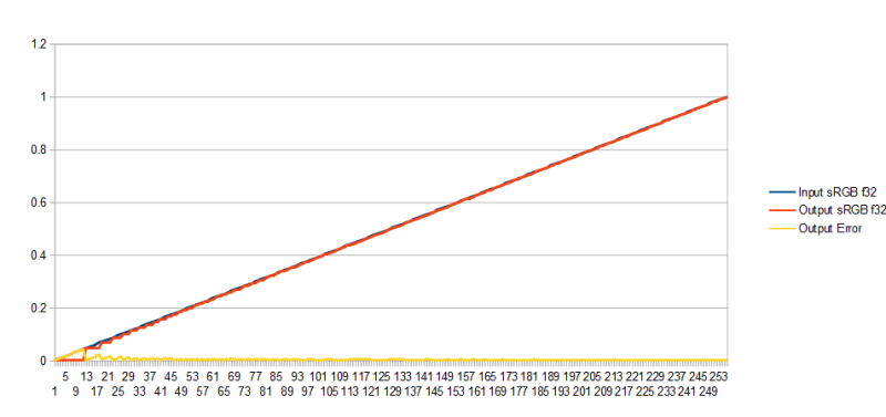
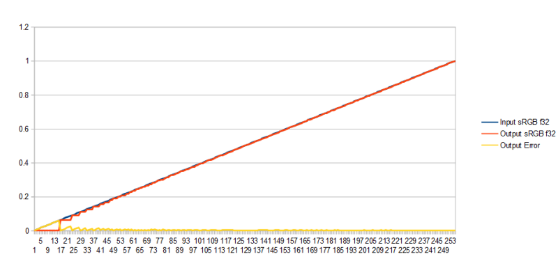
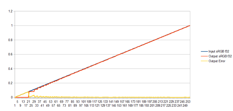
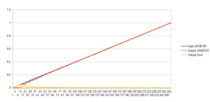
Here are some graphs to show the problem. Blue is the input color, red is the color after converting to linear u8, and then back to sRGB u8. Yellow is the difference between the two. (If wondering why I’m showing round trip instead of just 1 way, think about what you are going to do with the linear u8 image. You are going to use it for something, then convert it back to sRGB u8 for the display!)

Gamma 1.8

Gamma 2.0

Gamma 2.2

sRGB

As you can see, there is quite a bit of error in the lower numbers! This translates to error in the darker colors, or just any color which has a lower numbered color component.

The largest amount of error comes up in gamma 2.2. sRGB has lower initial error, but has more error after that. I would bet that was a motivation for the sRGB formulas, to spread the error out a bit better at the front.

Even though gamma 2.2 and sRGB looked really similar in the green to red color interpolation, this shows a reason you may prefer to use the sRGB formulas instead.

Another way of thinking about these graphs is that there are a quite a few input numbers that get clamped to zero. At gamma 1.8, an input u8 value of 12 (aka 0.047) has to be reached before the output is non zero. At gamma 2.0, that value is 16. At gamma 2.2 it’s 21. At sRGB it’s 13.

Showing graphs and talking about numbers is one thing, but looking at images is another, so let’s check it out!

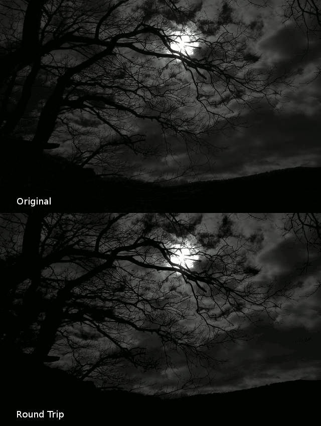
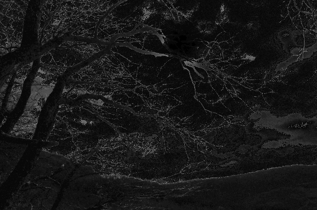
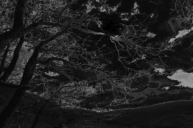
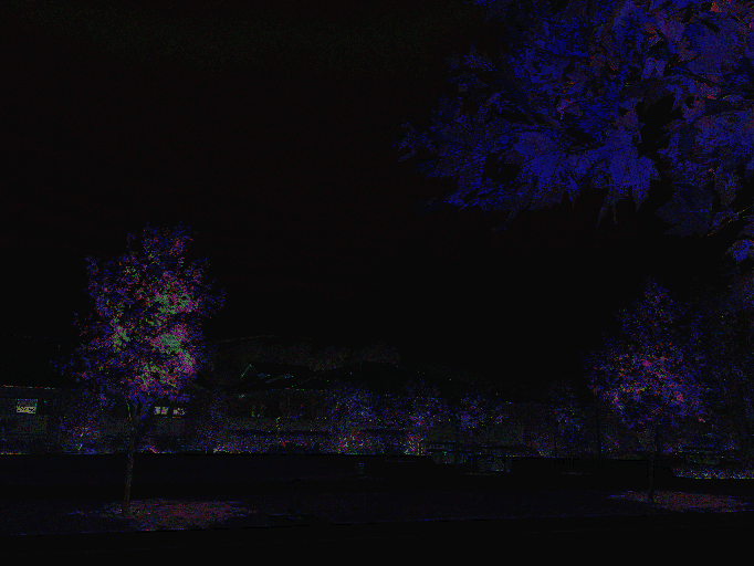
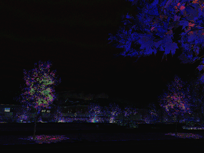
Below are images put through the round trip process, along with the error shown. I multiplied the error by 8 to make it easier to see.

Gamma 1.8

Gamma 1.8 isn’t the most dramatic of the tests but you should be able to see a difference.

Error*8:

Gamma 2.0

Gamma 2.0 is a bit more noticeable.

Error*8:

Gamma 2.2

Gamma 2.2 is a lot more noticeable, and even has some noticeable sections of the images turning from dark colors into complete blackness.

Error*8:

sRGB

sRGB seems basically as bad as Gamma 2.2 to me, despite what the graphs showed earlier.

Error*8:

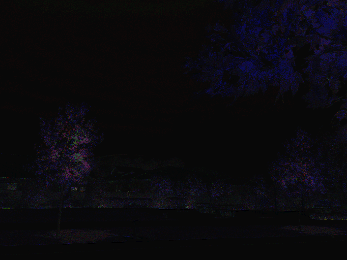
Since this dark image was basically a “worst case scenario”, you might wonder how the round trip operation treats a more typical image.

It actually has very little effect, except in the areas of shadows. (these animated gifs do show more color banding than they should, and some other compression artifacts. Check out the source images in github to get a clean view of the differences!)

Gamma 1.8

Error*8:

Gamma 2.0

Error*8:

Gamma 2.0

Error*8:

sRGB

Error*8:

So What Do We Do?

So, while we must work in linear space, converting our sRGB u8 source images into linear u8 source images causes problems with dark colors. What do we do?

Well there are two solutions, depending on what you are trying to do…

If you are going to be using the image in a realtime rendering context, your API will have texture format types that let you specify that a texture is sRGB and needs to be converted to linear before being used. In directx, you would use DXGI_FORMAT_R8G8B8A8_UNORM_SRGB instead of DXGI_FORMAT_R8G8B8A8_UNORM for instance.

If you are going to be doing a blur or generating mip maps, one solution is that you convert from sRGB u8 to linear f32, do your operation, and then convert from linear f32 back to sRGB u8 and write out the results. In other words, you do your linear operations with floating point numbers so that you never have the precision loss from converting linear values to u8.

You can also do your operations in u16 instead of u8 apparently, and also f16 which is a half float.

The takeaway is that you should “never” (there are always exceptions) store linear color data as uint8 – whether in memory, on disk, or anywhere else.

I’ve heard that u12 is enough for storage though, for what that’s worth.

Links Etc

Thanks @romainguy for suggesting a color interpolation for the opening image of this post. It’s a great, simple example for seeing why sRGB vs linear operations matter.

Here is some more info on sRGB and related things from Bart Wronski (@BartWronsk):

Part 1 – https://bartwronski.com/2016/08/29/localized-tonemapping/

Part 2 – https://bartwronski.com/2016/09/01/dynamic-range-and-evs/

And this great presentation from Timothy Lottes (@TimothyLottes)

Advanced Techniques and Optimization of HDR Color Pipelines

This from Matt Pettineo (@MyNameIsMJP) is also very much on topic for this post:

https://www.gamedev.net/forums/topic/692667-tone-mapping/?page=3&tab=comments#comment-5360306

Granular Audio Synthesis

If you want to make a sound shorter, you can play it faster. Doing this also makes it higher pitch unfortunately.

If you want to make a sound longer, you can play it more slowly. This also makes it lower pitch though.

Sound length and pitch are tied together and there’s no way to change one without changing the other.

… Actually that’s a lie. Granular synthesis can be used to change playback speed and pitch independently!

This post talks about how granular synthesis works, gives some examples you can listen to, and also supplies simple standalone C++ code that does it. (680 lines of code, one source file, only standard C++ includes, no libraries used.)

By the end of this post, you should even be able to program your own “autotune” effect.

The code and audio samples are available on github here: https://github.com/Atrix256/GranularSynth

Granular Synthesis Basics

Granular synthesis is conceptually pretty simple. The first step is to break a sound file up into small sections of sounds called “grains” that are typically between 10 and 100 milliseconds long.

You don’t have to do anything special to make grains, you just literally cut the sound up into a bunch of pieces.

To make a sound twice as long, you then make a new sound where each grain is repeated twice. When you play it back, it will sound mostly the same and be the same pitch, but will be twice as long.

To make a sound half as long, you would just throw away every other grain. The result is a sound that mostly sounds the same, and is the same pitch, but is half as long.

You aren’t restricted to integers though. You could easily throw out every 3rd grain to make it 2/3 as long or repeat every 5th grain to make it 20% longer.

You can also adjust pitch instead of length.

To make a sound that is the same length, but has twice as high pitch, you would double each grain, but play them back twice as fast. That would result in a sound that was the same length but had frequencies that were twice as high.

To make a sound that is the same length, but had half as high of a pitch, you would throw out every other grain, but play the ones you kept twice as slowly. That would result in a sound that was the same length but had frequencies that were half as high.

Congratulations, you now understand granular synthesis!

There are other usage cases of granular synthesis, but they are a lot more exotic – like making crazy cool sounds.

There are also variations of granular synthesis where grains overlap instead of being omitted, when dealing with sounds getting shorter, or grains being played a non integer number of times.

Check out this youtube video to see an insane usage case for real time granular synthesis. WTF!
Youtube: Drum Sound Experiment – Dynamic Granular Synthesis

Some Granular Synthesis Gotchas

If you just do the above, you are going to have some issues with clicking and popping. When you put grains next to each other that weren’t next to each other before, there is going to be a discontinuity in the audio wave form, which translates into very short, very high frequencies that make a popping noise.

What’s more is if your grain size is 20 milliseconds, that means you will get a pop 50 times a second, which means you’ll get a 50hz tone from the popping.

So, how do you fix this?

One way is to use envelopes to do cross fading.

If you wanted to put down grain A and then grain C that would make a pop because A and C expect B to be between them.

Using an envelop to fix this problem, you’d put down grain A, and then next to it you’d put down grain B but have it’s volume go from 1 to 0 over some length of time (like 2 milliseconds). You then ADD grain C on top of grain B, but have it’s volume from from 0 to 1 over the same length of time.

The result is that there is no immediate “pop” from discontinuous wave forms. Instead, it gently fades from one grain to the next over the length of the cross fade.

Note that the above is equivalent to linearly interpolating from grain B to grain C over the length of the envelope, it’s just done in two passes.

I’ve heard that another way to handle this problem is that instead of cutting grains perfectly at the time / length they should be at, you make the cuts at zero crossings that are closest to the desired cut position.

What this does is make it so you can put any grain next to any other grain, and they should fit together pretty decently. This gives you C0 continuity by the way, but higher order discontinuities still affect the quality of the result. So, while this method is fast, it isn’t the highest quality. I didn’t try it personally, so am unsure how it affects the quality in practice.

Another issue you will encounter when doing granular synthesis is wanting to play back a grain at a non integer playback speed. This means you may want to sample index 0, then index 1.1, then index 2.2 and so on. How do you sample a fractional index?

A quick and easy way is to use the fractional part of the index to linearly interpolate between the two samples it’s in between. That means that sampling index 2.2 would be a linear interpolation between index 2 and index 3, and would be 20% of the way from index 2 to index 3. AKA it would be value[2] * 0.8 + value[3] * 0.2;

Another way to sample fractionally is to use cubic hermite interpolation. It’s more expensive to compute but interpolates more smoothly, and perserves first order derivatives.

You can read more about that on my blog post here: Cubic Hermite Interpolation

Lastly, there are a couple parameters to these techniques that have to be hand tuned for the situation they are used in:

  • Grain Size – Some usage cases want larger grain sizes, while others want smaller grain sizes. You’ll have to play with it and see what’s best for your usage case. Again, I’ve heard that typical grain sizes can range between 10 and 100 milliseconds.
  • Envelope Size – The size of the envelope used for cross fading can affect the result as well. Too short an envelope will start to make popping happen, but too long an envelop will muddy your sound.

Drums and other percussion instruments have a particularly hard time with granular synthesis because they are usually made up of very short but noticeable sounds. If these sounds get (partially?) repeated, it will sound weird and wrong.

Check the links at the end of the post for deeper reads into these topics and more!

Experiments & Results

For all experiments, I used a sound clip from one of my favorite movies “Legend” where Tim Curry plays the devil, and Tom Cruise and Mia Sara are the main characters fighting him.

legend1.mp3:

The experiments use cubic hermite interpolation to sample fractionally, and they use crossfading to fight popping between grains. Everything uses a grain size of 20 milliseconds, and a cross fade of 2 milliseconds.

Naive Pitch / Length Adjustment

To start out, we can play the sound faster and slower to naively adjust pitch and length.

Here’s a fast / high pitched version (70% of time):

Here’s an even faster / higher pitched version (40% of time):

Here’s a slow / low pitched version (130% of time):

And here’s an even slower / lower pitched version (210% of time):

Granular Synth Length Adjustment

Here is a sound made shorter (70% of time) using granular synthesis, so is the same length as the fast/high version, but has the same pitch as the original. Pretty cool, right?

Here is the sound made even shorter (40% of time) so is the same length as the faster/higher version, but has the same pitch as the original again.

Here is the sound made longer (130% of time), but again has the same length as the original.

And here is the even longer version (210% of time).

Granular Synth Pitch Adjustment

If we want to adjust the pitch but leave the length alone, there are two ways you could do that.

The first way is to use granular synthesis to change the length of the sound (longer or shorter), keeping the pitch the same, then use the regular “naive” method to make that resulting sound be the original sound length again.

If you made the sound shorter to start with, this process would decrease the pitch. If you made the sound longer to start with, this process would increase the pitch.

Here is a sound where that process is used to make the pitch about 1.43 times higher (1.0/0.7), but keeps the same sound length.

Another way to get a very similar result is to just change the playback rate of the grains themselves – INDEPENDENTLY of how many times you repeat the grains (0 to N times) which changes sound length.

Here is a sound made doing that. It plays each grain back ~1.43 times faster, but makes a sound that is the same length in the end. My ears can’t tell the difference, even though I do know there is one. This is the technique we’ll be using for the rest of the experiments.

Here is a higher pitched sound that plays back each grain 2.5 times faster (1.0 / 0.4).

You can use this to make the sound lower pitched as well. Here is a sound where we play the grains back at 0.77 speed (1.0 / 1.3).

Here they play back at 0.48 speed (1.0 / 2.1).

Granular Synth Pitch and Length Adjustment

To really drive home how pitch and length adjustments can be made independent with granular synthesis, here is a sound where it plays back more slowly (130% as much time), but it plays back at a higher pitch (~1.43 times as high).

And the opposite… here is the sound played back more quickly (70% as much time), but it plays back at a lower pitch (~0.77 times as high)

Dynamic Parameters

Something else fun is that the parameters don’t have to be fixed at runtime.

In the example code, I have a version of the granular synthesis function that calls back to a lambda for every grain to see what time and pitch multiplier it should use.

Here the pitch is on a 10 cycle sine wave going between 0.75 and 1.25.

Here the sound length is on a 13 cycle sine wave going between 0.5 and 2.5.

And lastly, here it combines the pitch and sound length parameters described above.

Links

Below are some great links for more information about granular synthesis. I also recommend searching youtube for “granular synthesis examples” to hear some really out there stuff.

https://www.soundonsound.com/techniques/granular-synthesis

https://granularsynthesis.com/guide.php

https://theproaudiofiles.com/granular-synthesis/

I also want to mention that the basics of this technique was kindly described to me at lunch by a co-worker. His web page is at http://antonte.com/