There is an interactive demo that goes with this post where you can play with filter parameters, hear the resulting filter applied to audio samples, and copy/paste the simple formula to use the filter in your own applications:
Finite Impulse Response Filtering.
There is also some simple standalone C++ code (~170 lines) that shows how to apply filters, as well as calculate phase/frequency response and zero locations:
https://github.com/Atrix256/DSPFIR
The math behind frequency filters can look pretty daunting, but it’s actually not that bad!
This post is going to talk about a simple, real time friendly filter called a “Finite Impulse Response” or FIR filter. They are also known as feed forward filters.
An order 1 FIR filter looks like this:
 is the filtered sample,
  is the current unfiltered sample,
  is the previous unfiltered sample, and
  and
and  are values to multiply the samples by to control the filtering.
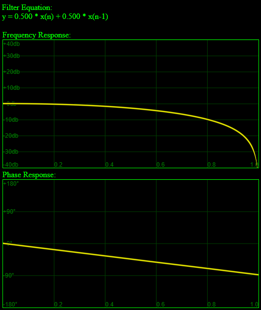
For instance, the below averages the samples, which is also called a box filter. This is in fact a low pass filter, meaning that it filters away higher frequencies while letting low frequencies pass through.

If you change the addition to a subtraction, you get a high pass filter, which filters out low frequencies, and lets high frequencies pass through.

An order 2 FIR filter looks like the below and the pattern continues for higher order filters.

These equations are called difference equations and this post is going to show you how to analyze them to understand what they do, and how to craft your own that behave in specific ways.
Gain Parameter
If you made a machine that applied an order 1 FIR filter, where you gave a knob to control and , you’d find that the knobs were pretty unintuitive.
Specifically, if you had the knobs set to a specific setting that you liked, but you wanted the overall filtered sound to be louder or quieter, it would be difficult to make that happen. (spoiler: the ratio between them would need to stay the same but if you made them larger magnitude numbers the result would get louder)
This problem only gets worse with higher order filters as you add more knobs.
To deal with this, you can factor out the parameter which makes the order 1 equation into the below:

We can replace  with
with  to get this equation:

Now, you can have two knobs for those two parameters and things are much easier to deal with. You can adjust to adjust the volume, and you can adjust to adjust how frequencies are affected by the filter.
If you wanted to get out again, like for use in the difference equation, you would just calculate it like this:

You can do the same process to the order 2 FIR filter to get this equation:

where

and

From Difference Equation to Transfer Function
The difference equation is how you filter data, but it doesn’t really help you understand what the filter is actually doing.
To understand what the filter does, and how it affects various frequencies, we need something called a transfer function. We can transform a difference equation into a transfer function with a handful of steps.
First, instead of putting a signal through our filter, we need to put through a complex sinusoid  , which will let us plug in different frequency values for omega (
 ) to see how the filter affects those frequencies.
While we can replace with , what do we replace with? We replace it with  . Another way to write that is
  . That shows that we can multiply any point in our complex sinusoid signal by
  to get the previous sample, which is super handy, as it delays the signal by one sample.
So, let’s go back to our difference equation and plug in the complex sinusoid.
Then let’s factor out the complex sinusoid.

That sinusoid is what we input into the equation so we can replace it with  .
.

The transfer function is  divided by so let’s put it in that transform function form:

The next step is to do a replacement in the function. We are going to define  , which makes our transfer function look like the below.

We are done! That is the transfer function of our order 1 FIR filter which is controlled by two parameters:
- – This is the gain (volume) of the filter
- – This controls how the frequencies are filtered. Multiply this by to get the parameter if you ever want to (like to use in the difference equation), but let the user control this value directly.
For order 2, if we do the same, we end up with this equation:

The parameters are the same but order 2 adds in a  which also controls how the frequencies are filtered. You can also multiply by if you want to calculate the
  value for use in the difference equation.
Complex Sinusoids, Complex Unit Circle, Phase and Frequency Response
There’s a bizarre looking equation called Euler’s identity which looks like this:

This is actually just a specific value (pi) plugged into the more general Euler’s formula:

In those formulas, you can see that x is an angle, so when you plug in pi, you are plugging in 180 degrees. The result you get out is a complex number where the real part is the cosine of the angle, and the imaginary part is the sine of the angle.
The cosine of pi is -1, and the sine of pi is 0, so that’s why Euler’s identity gives you -1 as a result. It’s really -1 + 0i.
Something interesting you may remember is that if you want to draw a point on a unit circle, x is cosine theta, and y is sine theta. (Theta being the angle from the origin to the point)
So, what this tells us is that Euler’s formula is a way of drawing a circle where the x axis is the real number axis, and the y axis is the imaginary number axis.
In the last section, we plugged a similar looking – but different – complex sinusoid into the equation that looked like this:
The difference is that we have omega times t as our x value.
t is the time variable, so is what we increase to move around the circle.
Omega says how many radians around the circle the point travels every time t increases by 1.
If omega is zero, that means the point is stationary and doesn’t move. It also means it has a frequency of zero. This is 0hz or DC.
If omega is pi/2, that means the point moves pi/2 radians (90 degrees) around the circle every time t increase by 1. If this were a cosine wave, and t was an integer index for samples, it would repeat: 1, 0, -1, 0. This is also 1/2 nyquist frequency.
if omega is pi, that means the point moves pi radians (180 degrees) around the circle every time t increase by 1. As a cosine wave it would repeat: 1, -1. This is nyquist frequency.
Anything higher frequency than nyquist has aliasing problems and can’t be reconstructed from the samples, so it makes sense to stop there.
Similarly, if at 0 radians, you go negative, such as -pi/2, that is the same as 3*pi/2 which is above nyquist, so we stay away from the negative frequencies as well.
In any case, we are plugging a circle into the transfer function where the angle on the circle just means “how many radians does this wave form advance each sample”, and as output, we get that circle but distorted. A filter where output = input without any filtering happening would leave the circle unaffected.
The output point for a given input point is another point on the complex plane (x = real, y = imaginary).
The distance of this point from the origin (or, the magnitude of this vector) tells us how much the amplitude (volume) would be altered for a signal with that frequency. A value less than 1 means that it gets smaller/quieter, while a value greater than 1 means that it gets larger/louder.
The angle that the output point is on the circle (use atan2 to get this value) tells you how much this signal will be “phase shifted” or how much it will be delayed. For instance, if the signal is advancing at 90 degrees per sample, and it has a phase shift of -90 degrees, that means the signal is effectively delayed by 1 sample. A positive phase shift means that the signal is moved forward in time, and is an anti-delay (it’s from the future kinda).
This stuff is all very interesting, because real signals / sounds are commonly made up of several different frequencies. The filter treats all those frequencies independently and does the things it says it will – as far as wave amplitude and phase shift – to each frequency that may be present, independent of what it does to the other frequencies.
Frankly, it feels a bit magic that it’s able to do that, but that’s what it does.
You can actually plug angles between 0 and pi into the transfer function, get complex numbers out, calculate the amplitude and phase response, and graph them. This gives you something where you can see how a filter actually behaves. We do 0 to pi, because that is 0hz to nyquist.
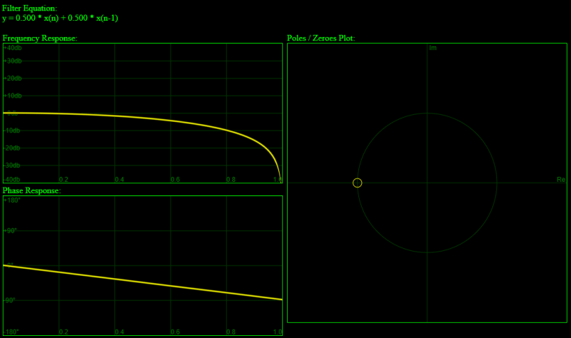
Below is the before mentioned “box filter” aka low pass filter, that you get when you average the current sample with the last. You can see that the low frequencies are left alone (0db) but that higher frequencies drop down in amplitude a lot as they approach nyquist. The x axis labels are % of nyquist, so at the very right is the nyquist frequency – the highest frequency that is able to be expressed.
Note: this and the other screenshots came from the interactive demo that goes with this post. You can find it at http://demofox.org/DSPFIR/FIR.html
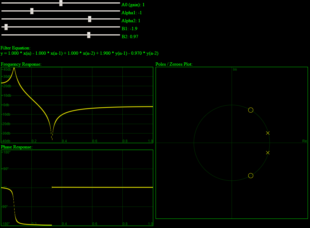
Pole Zero Plot of Order 1 FIR Filter
Lets take a look at the transfer function of our order 1 FIR filter again:
Now i have a question for you… what value(s) of z make this function equal to zero? You can work through some simple algebra to find that it’s where  :
:

This just means that on the complex plane, the function equals zero at that location.
As points in the function get closer to there, they will approach zero as well.
What this means is that frequencies on the complex sinusoid unit circle that are nearer to this zero will be attenuated (shrunken, made smaller / quieter), while frequencies farther away won’t be, or won’t be attenuated as much.
So, you control what frequencies get filtered just by where the zero is!
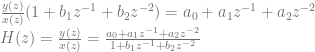
If the zero is on the left, at angle pi (180 degrees), where the highest frequencies live (nyquist!), the high frequencies will get attentuated, making it a low pass filter. Below is the box filter again, which does this.
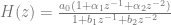
If the zero is on the right, at angle 0, where the low frequencies live, the low frequencies will get attenuated, making it a high pass filter.
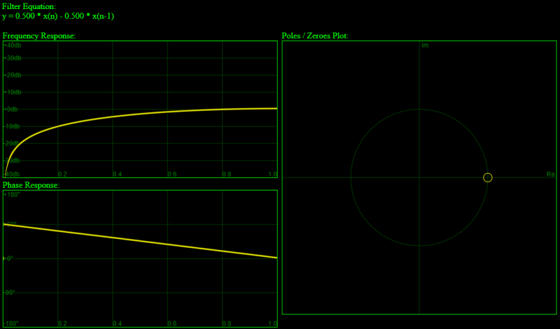
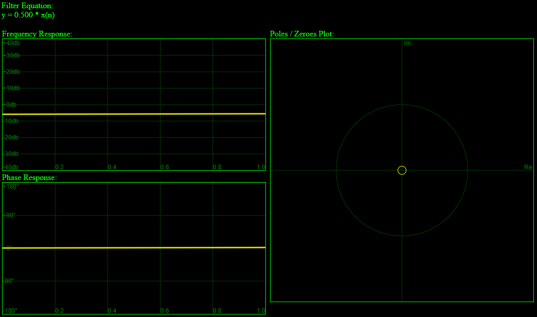
If you put the zero in the middle, you get a filter that doesn’t do anything, other than possibly a0 adjusting the volume, like in this filter.

You don’t have to keep the zero inside the unit circle though. Here it is going outside of the unit circle to the right. You can see that low frequencies are still attenuated, so it’s a high pass filter, but they are not attenuated as sharply.
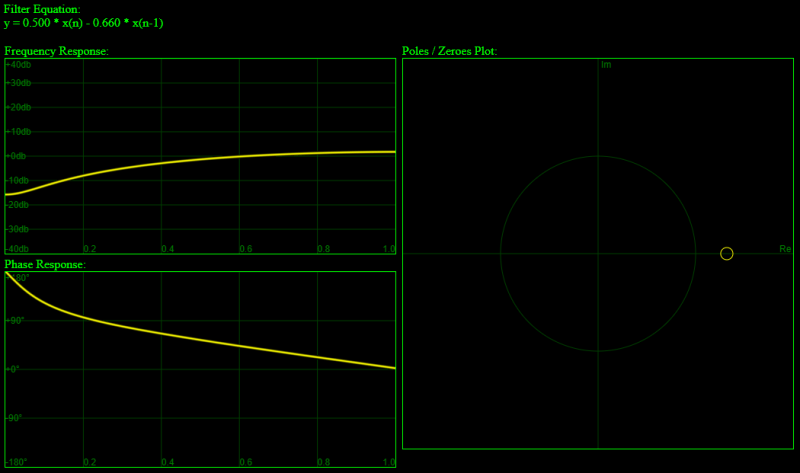
It’s also worth noting that the last filter was the first filter where the phase response was not a line. The other filters had “linear phase response”. Linear phase filters have some nice properties that are sometimes desired, such as not distorting the shape of a wave form, other than adjusting frequency amplitude.
You’ve now essentially seen everything that an order 1 FIR filter can do. There’s a zero you can move around on the real axis (the x axis) and any frequencies near the zero get quieter when passed through the filter.
It’s important to note that the zero can only make things quieter. This means that FIR filters are stable. They never suffer from feedback issues where they make something louder and louder and louder into infinity or start spitting out NaNs. That makes them pretty attractive if you really want a stable filter, but that stability is also tameness.
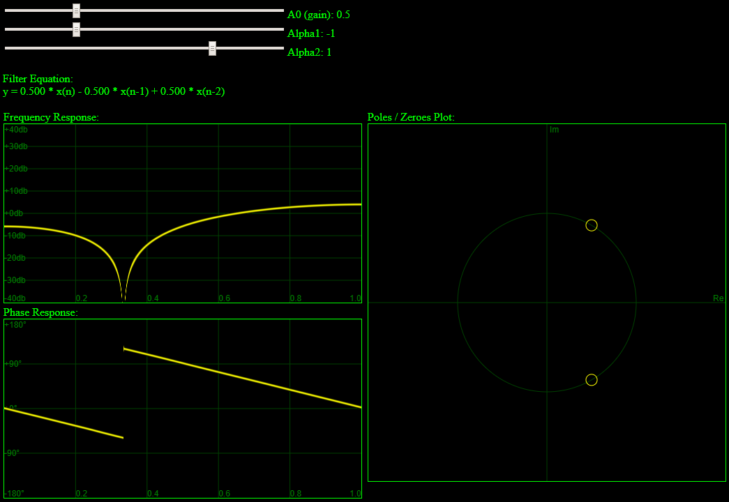
Pole Zero Plot of Order 2 FIR Filter
Let’s take a look at the transfer function of 2nd order filters.
Just like with the order 1 filters, we need to find out where the zeroes of the function are. With some algebra we can get it to something more manageable:
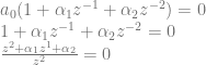
Looking at that, when z is 0 (the origin), it shoots to infinity. That’s called a “pole” which is the opposite of a zero. We’ll talk about them lots more in the next post, but for now, since it’s at the origin we can ignore it as a “trivial pole”.
So, we need to figure out when the top part of the fraction is equal to zero:

Luckily this is a standard quadratic polynomial, just like if we had 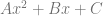 . In our case, x is z, A is 1, B is and C is .
To solve those equations we normally would use the quadratic equation:

For our purposes, it is more convenient to re-arrange that a bit to be like the below:

The reason for this is because we are going to have two zeroes (roots) when we solve this thing. The left side is the x axis (real axis) middle point between the two roots. The right side tells us how much to move on each side of that middle point to get to the zeroes. If the number under the square root is positive, it will give us a real number answer, that we will use to move left and right on the x axis. If the number under the square root is negative, it will give us an imaginary number answer, that we will use to move up and down on the y axis.
We can plug in our values for A, B and C and get our roots:

It isn’t as clear where the roots are as it was for an order 1 filter, but it will tell us where they are if we plug values in.
Firstly, the center between the zeroes will be at  . So, if is 1.0, the zeroes will be evenly spaced away from -0.5 on the real axis. If it’s -2.0, the zeroes will be evenly spaced away from 1.0 on the real axis.
From there, you just modify to change if the zeroes move on the real axis (x axis) or the imaginary axis (y axis) and by how much. Pro Tip: If you give a value of 1.0, the zeroes will be on the unit circle.
Here is an order 2 high pass filter:

Here is an order 2 low pass filter:
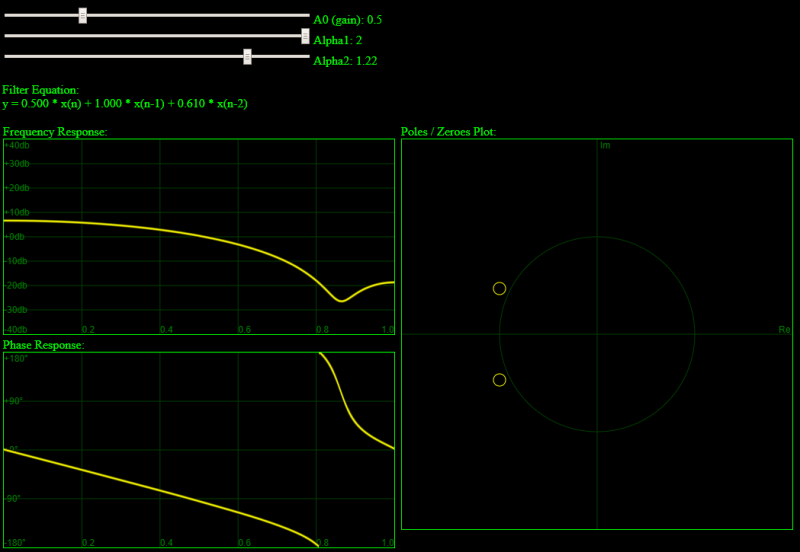
Lastly, here’s an order 2 notch filter, which means it cuts a “notch” out of the frequency spectrum. It can sound pretty cool to play a sound (in the acompanying demo) and slide the notch up and down the frequency range.

Estimating Frequency Response From a Pole Zero Plot
If you have a pole zero plot of an FIR, here is how you estimate how much a specific frequency will be attenuated by that filter.
Draw a line from that frequency on the unit circle to every zero on the plot and get the lengths of those lines.
Multiply all the length of the lines together.
That final result is an estimate of how much the amplitude of a sinusoid wave in that frequency will be attenuated.
A value smaller than 1 means it will get smaller (quieter) while a value greater than 1 means it will get bigger (louder).
I’m not sure why it’s only called an estimate though. When looking at order 1 and order 2 filters, I’ve been unable to find a situation where they don’t match visually. The demo has a checkbox at the bottom to draw the estimate in teal if you want to see for yourself.
Why is it Called Finite Impulse Response?
There is a concept of an “impulse” where you have a signal this is a bunch of zeroes, then a single 1, then a bunch of zeroes again. Putting an impulse through a filter is a way to analyze how a filter behaves, and in fact is a unique finger print for the filter which you can use to reconstruct the coefficients of the filter itself.
If it’s a finite impulse response filter, the impulse response is actually the coefficients of the filter itself, which is pretty nifty.
Let’s check out the difference function for an order 1 FIR:
In this situation we have only a couple cases to think about.
When we start in the “a bunch of zeroes” section of the signal, it’s going to be a0 * 0 + a1 * 0, which is always going to be zero.
So, for that part of the signal, we always have zeroes.
Then, we hit a point where is 1 and is 0. In this case, the output of the filter is going to be a0.
Next, we hit the point where is 0 again and is 1. In this case, the output of the filter is going to be a1.
Then, we have a bunch of zeroes again and the filter will keep putting out zeroes until the sun goes dark.
The fact that this filter had a “finite response” to the impulse, meaning it settled back down to zero and stayed zero, is why it’s named a finite response.
In contrast to this, if the filter had some kind of internal state that was updated as each sample went through, it could very well never go back to zero. In that case, we’d have an infinite impulse response or IIR. The next blog post is going to talk about that kind of a filter.
Crafting a Filter By Placing Zeroes
If you have a high order FIR – say an 8th order one – it’s very difficult to find the zeroes because you ultimately need to find the zeroes of an 8th order polynomial, which is not really possible analytically in the general case.
However, if you want to go the reverse way, where you have placed your zeroes in specific locations and want to make a filter from that, that is a lot easier.
First up, you need to decide where your zeroes are.
- You can have as many zeroes as you want.
- Duplicating zeroes make them have steeper attenuation, but also the effect is more localized and more distant frequencies are affected less than closer ones which are affected more.
- You can add as many real valued zeroes as you want.
- For every complex zero you add, you also need to add it’s complex conjugate. For instance, if you add 1+3i, you also need to add 1-3i. If you don’t do this, your filter can spit out complex numbers instead of only real numbers!
To work through an example, let’s say that we have 4 zeroes: 3, -2, 3i, -3i.
First we need to make a polynomial with those zeroes.
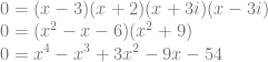
Next, we could work through some simple algebra (the reverse of what we did in previous sections), but to jump straight to the punch line, our filter coefficients are the coefficients of this polynomial: 1, -1, 3, -9, -54. That gives us this difference equation:

Or simplified:

If you want a gain parameter in your filter function, just multiply all the coefficients by that value.
You can also use those coefficients to go directly to the transfer function very similarly. The coefficients are inside the parens.

Or simplified:

Before moving on, it’s important to note that some coefficients may be zero and you need to watch out for that. For instance, let’s say you have zeroes at +/- i:

You would probably be tempted to say that the filter coefficients are “1, 1” (I made that mistake!) but in fact, they are “1, 0, 1”. The equation above is really this one below:

Making Cool Sounds & Music
A really fun thing to do in the demo (http://demofox.org/DSPFIR/FIR.html) is to make it play white noise and then filter the white noise. You can make it sound like wind or the ocean, or other things. White noise contains all frequencies so filtering like this can make some really interesting sounds. Some other types of sounds (like a sine wave tone) have only a single or very few frequencies, so putting them through filters doesn’t make them sound that interesting.
Filtering sounds to create new sounds is called subtractive synthesis (since you are attenuating or removing frequencies). It’s not something I’m very experienced at musically, but I’m finding that I really like the sound of making some frequencies become very loud and clip (causing distortion), while other frequencies do not. I anticipate the next post on IIRs will have more of that. IIRs place infinities (poles) on the pole zero plot so can boost frequencies quite high, instead of how FIRs can only place zeroes that make some frequencies quieter.
Here’s something to try in the demo…
- Have it play the harp sound clip
- Set it to an order 2 filter
- Turn on overdrive and set gain to 33
- A0 = 33, alpha1 = -1.34, alpha2 = 1.
- Bonus: slide alpha1 back and forth slowly. You could imagine putting that parameter on low frequency sine wave so that it did this part automatically.
You are on your way to making music! If that sounds awesome to you, you might like my other audio blog posts: https://blog.demofox.org/#Audio
Closing
Now that you understand how FIR’s work, you may be interested in a post i wrote about generating different distributions and colors of noise using dice. It turns out they are just FIRs in disguise. The dice are just a source of white noise and the operations with adding and subtracting is just having positive and negative coefficients in the filter 🙂
https://blog.demofox.org/2019/07/30/dice-distributions-noise-colors/
Also, something nice about FIR filters is that the filter is stateless. You just multiply the last N samples by N specific coefficients to get your result. This means you can apply a filter to a signal via convolution. Convolution isn’t a cheap operation, but it does a lot of simple branchless operations in parallel, which is something that things like GPUs and SIMD excel at. You can also use the convolution theorem by taking the signal and filter coefficients into frequency space (DFT via the FFT), multiplying them together, and taking them back into time space (IDFT via the FFT again). This can be more efficient for a high order filter. In fact, really nice reverb is made up of a very long impulse response, which makes it a very high order filter. It’s not uncommon to implement reverb via convolution (but doing it as a multiplication in frequency space).
I’d like to thanks these 3 peeps who helped me understand some DSP concepts. Thanks for your kindness!
@BartWronsk
@nickappleton
@rygorous
Also, this book is exceptional as an introduction to DSP, specifically meant for audio purposes. It has dsp theory but also information about how to program things like compressors and limiters, flange, chorus and reverb. It’s very cool and a lot of fun.