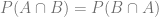
Thank you Uncle Chris and Aunt Lily for sending me this gigantic 120 sided dice!
A while back I came across an interesting page that talks about some fundamental concepts relating to noise. It isn’t very long or hard to read, but has some great info.
Dither noise probability density explained
https://www.digido.com/ufaqs/dither-noise-probability-density-explained/
The main points it makes are:
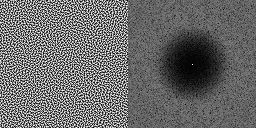
- White noise just means the noise values are drawn independently and have no correlation to each other. Blue and red noise (and other noise colors) are correlated samples.
- The distribution (histogram) the values are generated / drawn from is completely unrelated to the “color”.
I wanted to go through the experiments it mentioned to understand what it was talking about a bit better. This post does that and explores a few other related experiments and algorithms.
You can find the code that goes with this at https://github.com/Atrix256/NoiseDims
Intro Image Explanation
Thanks to my Uncle Chris and Aunt Lily for sending me that gigantic 120 sided dice. That thing is epic.
You’d need to roll those 20 dice next to it to equal the massive THAC0 power than it has. But as you’ll see in this post, doing so would give you a Gaussian distribution, and not all numbers would come up with equal probability or even be possible. Try rolling a 1 with 20 six sided dice!
The black dice in the background are some cool diablo themed dice I got one year from Blizzcon.
Seeing as the dice are not magnetic, or quantumly entangled, rolling these dice should give you uncorrelated values (white noise), but I can’t vouch for their histograms (are they fair dice or not?).
BTW i am taking this picture from inside my hotel room in LA during SIGGRAPH, instead of going out and being social. This is what real programmers do right? Ditch social engagements to take pictures of dice and compare histograms and DFTs? This post has been sitting in my drafts for far too long and just really needed to get finished 😛
Onto the post!
Testing Methods
There are two main tools used in this post to understand noise patterns better.
The first is the histogram:
You do your process N times to get N random numbers and keep track of how many times each number came up. For a small number of rolls, the histogram will likely be erratic, but for a larger number of rolls, it will take the shape of the distribution of the numbers.
The second is the magnitude component of the Fourier transform of the rolls:
You do your process N times to get N random numbers. Do a discrete Fourier transform of that sequence of numbers to see the frequencies involved and extract the magnitude of each frequency (ignoring the phase). Just like the histogram, A small number of rolls will likely be erratic, but a larger number of rolls will show more clearly the actual frequencies present in the number sequence.
So in short: The histogram shows the distribution, and the Fourier transform shows the noise color.
White Rectangular Noise
White rectangular noise is “regular old random numbers”. Roll a die, write down the value. Rinse and repeat.
It has the properties that…
- The samples have no correlation to each other.
- Every possible value has the same probability of being chosen.
The example code rolls a 6 sided dice a number of different times. Here is the result it gets for rolling the dice 16 times:
2, 0, 2, 2, 0, 3, 2, 4, 2, 2, 0, 5, 0, 3, 1, 3
There sure are a lot of 2’s aren’t there? You might not look at this sequence and think it’s very random, but it is.
This is just how white noise works; it has clumps and voids and is in general pretty uneven.
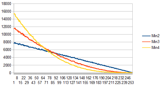
At the limit (large sample counts) it evens out. Check out the image below to see how the histogram gets flatter as the number of rolls gets higher. This shows that it is a rectangular distribution. (Note: The 8192 x 100 line is the average of 100 different 8192 runs)

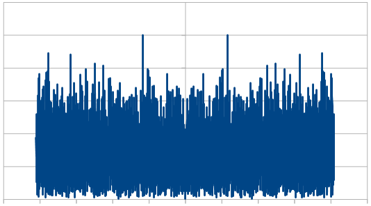
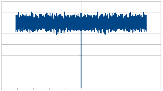
From a frequency point of view, since it’s white noise, it should have all frequencies present in equal amounts.
At 16 samples, the frequency magnitudes are a bit wild:

At 1024, they are flattening a bit:

At 8192, even more so:

When averaging 100 runs of 8192, it cleans up a lot and shows roughly the same magnitude for all frequencies, which shows that the noise color is white and the rolls are uncorrelated.

White Triangular and Gaussian Noise
If you roll two dice and add them, you get white triangular noise. You can also subtract one from the other and get white triangular noise.
If you involve more than two dice and do additions and subtractions of various amounts, the triangle rounds out and starts to look more like a normal aka Gaussian distribution. If you rolled an infinite number of dice, it would be Gaussian. This is due to the central limit theorem (https://en.wikipedia.org/wiki/Central_limit_theorem)
Doing these things, the dice rolls are not correlated with each other so they are still white noise.
Adding two dice (0-5) together, gives a result 0-10. Here’s the histogram of 1024 rolls:

Averaging 100 different 8192 sets of rolls gives this much cleaner histogram:

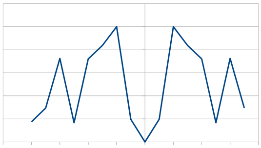
And when looking at the frequencies (averaging 100 different 8192 rolls), it still looks white, despite having a different histogram / distribution.

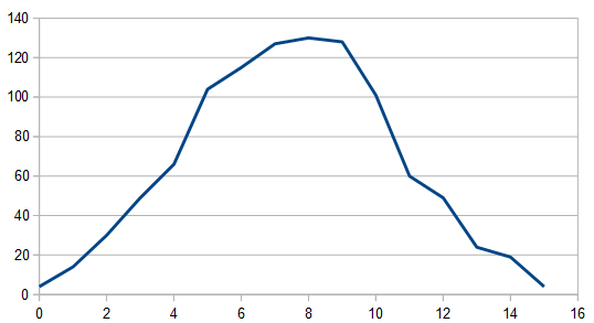
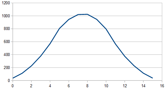
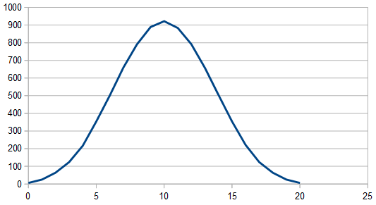
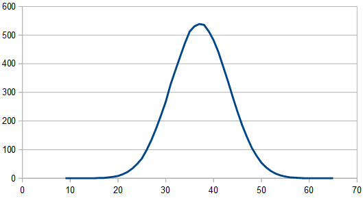
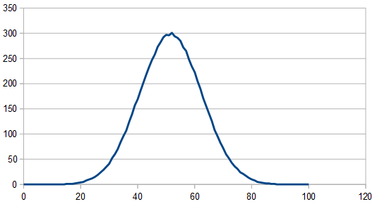
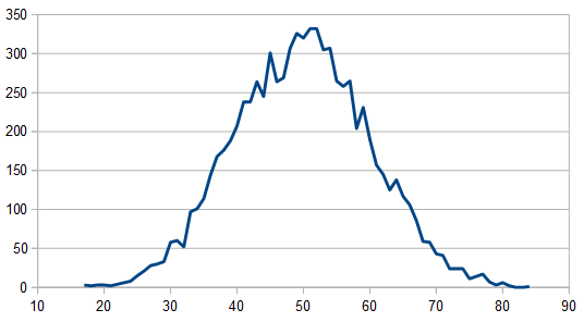
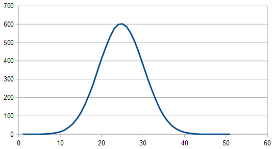
Adding three dice together gives results 0-15. The histogram for 1024 rolls still looks pretty lumpy:

But it cleans up when averaging 100 different 8192 rolls and looks pretty gaussian, since there are 3 dice involved instead of only 2.

The frequencies look the same (white) so I won’t even bother showing them.
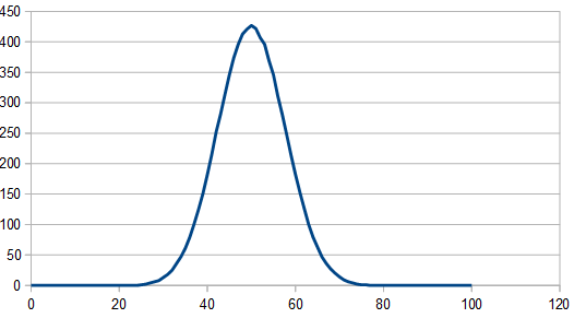
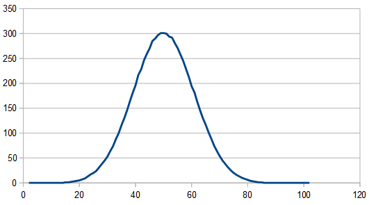
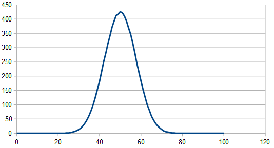
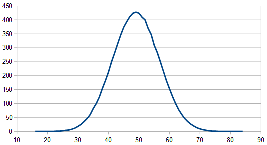
Here’s the histogram of 100 different 8192 rolls, using 20 dice each roll and summing them up. The frequencies look white still, so i won’t bother showing them.
Rolling two dice and subtracting one from the other looks the exact same as adding them together, except the histogram goes from -5 to +5, instead of from 0 to 10.
You can generalize this subtraction to a larger number of dice by summing up all the dice, but multiplying half of them by -1 before doing the summing.
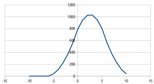
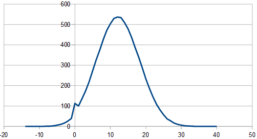
If doing an odd number of dice in this setup, it looks different in that one side of the Gaussian tail is chopped off, like below, but still looks white in frequency space. 3 dice were used here, where two dice were multiplied by -1 before summing.

Sure you can roll a lot of dice and add them together to get white Gaussian noise, but you can also generate Gaussian numbers directly (check this out to see one way: https://en.wikipedia.org/wiki/Box%E2%80%93Muller_transform). If you do this and write down the numbers, the histogram looks Gaussian as you’d expect, and amazingly (or not amazingly), it still looks perfectly white in frequency space. I won’t bother showing the images, but I did write the code for it and verify, so you can check out the output of the code that goes with this post for yourself if you’d like!
Red Triangular and Gaussian Noise
Let’s say you roll two dice and add them up. This is triangular white noise like we saw above.
If you name your dice A and B, you can now reroll A and add them again to get the second number. You then reroll B and add them again to get the third number. You then reroll A and add them again to get the fourth number, and so on. This is triangular red noise!
By only rerolling one of the dice, you are low pass filtering the white noise and getting red noise.
In more plain terms, by only re-rolling one of the dice each time, the sum is going to tend to be more similar to the last sum. That makes for random numbers that have stronger low frequency components.
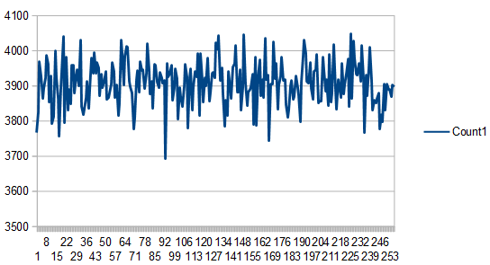
Here are the results from the program of doing this 16 times:
2, 4, 2, 3, 5, 6, 6, 4, 2, 5, 5, 3, 4, 4, 8, 7
As you can see, the numbers are usually pretty similar to the numbers around them, which is different than the white noise case. This is red noise.
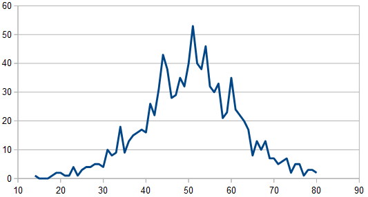
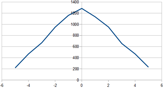
Doing this 8192 times, the histogram looks like a wiggly triangle as the image below shows, but averaging 100 runs of 8192 samples, it looks like a perfect triangle (not shown).

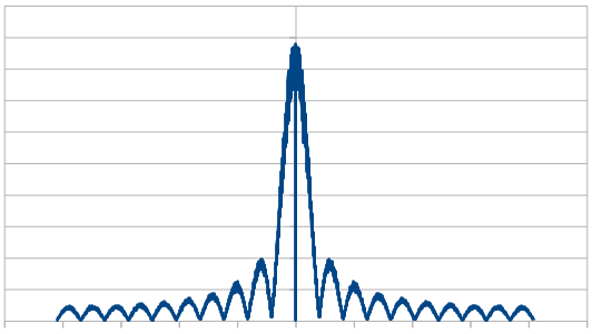
Looking at it in frequency space, here’s 16 samples:
1024:

8192:

8192 x100 averaged:
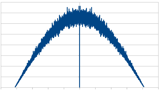
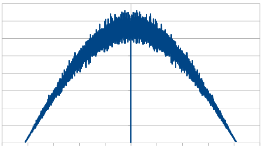
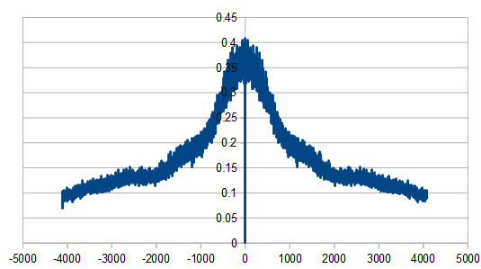
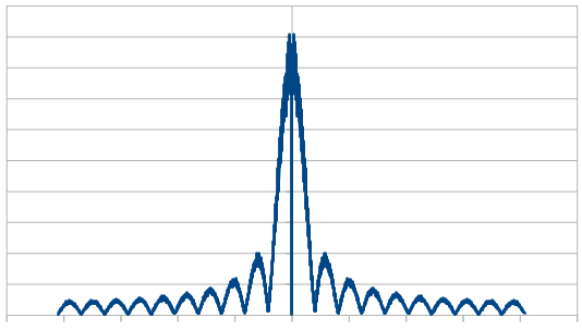
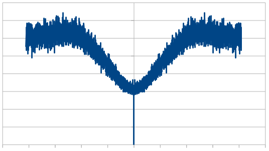
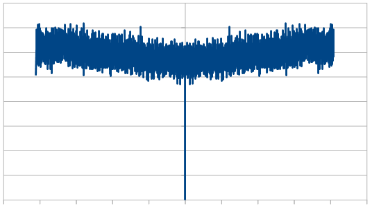
So, the histogram shows a triangular distribution, and the frequency space shows low frequency content – the part in the middle is the low frequencies and that’s where all the amplitude is. We have triangular red noise!
What if we use a different number of dice?
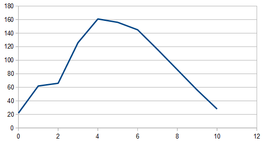
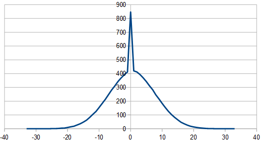
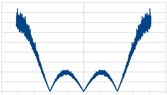
Here is the histogram and DFT for having 3 dice, and rerolling one each time (cycling through which die is rerolled). These are the averaged 8192 x100 rolls. The histogram shows a more gaussian distribution, and something odd is going on with the frequencies.

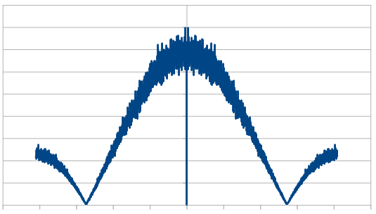
Here is the same for 4 dice.

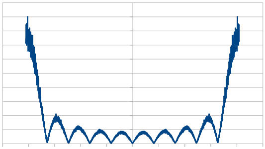
Here it is for 10 dice.

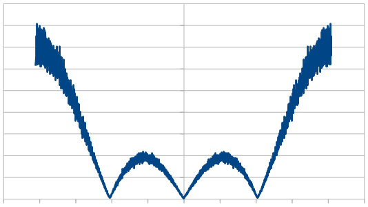
And here it is for 20 dice.

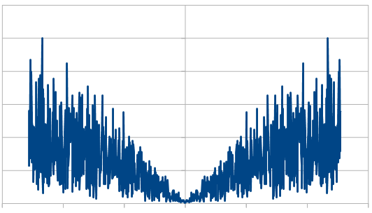
So, as we use more dice, the histogram gets more Gaussian, but for every dice added, we also get “half a hump” in the frequency space. The noise is undeniably red though, as the largest peaks are in the middle, where the low frequencies are.
If you are curious, here’s 16 rolls of 20 dice being used to make red noise, which means only re-rolling one dice each roll. It is very “random walk”-ish and the numbers don’t stray too far from 50, which is the expected value.
49, 49, 51, 51, 53, 55, 56, 55, 54, 54, 57, 57, 62, 61, 61, 62
You might think that those numbers are on their way up, but here are the next 16 values it gives to show you that isn’t the case.
59, 59, 57, 52, 51, 55, 55, 54, 55, 51, 52, 53, 57, 58, 59, 58
All this time, we’ve only been rerolling one die. What if we re-roll a different number of dice?
Here we roll 20 dice, but reroll 5 each time (cycling through the dice). We did this 8192 times, and averaged the results of doing that 100 times. In frequency space it looks a lot like our 4 dice case. I guess that isn’t too surprising if you think about us re-rolling 1/4th of the dice in both cases.


Here we reroll 10 dice each time. In frequency space it looks like when we rolled 2 dice. Again, maybe not surprising, because we are rerolling 1/2 of the dice now just like before. We do get the nicer Gaussian distribution though of using 20 dice though.


Rerolling 15 dice each time, the histogram is unaffected, but here are the frequencies:
Here we reroll 19 dice:
So, taking some empirical observations it looks like when summing dice…
Using more dice makes the distribution more Gaussian (thanks central limit theorem!)
Rerolling less of the dice each time makes for stronger low frequency content, while rerolling more dice makes the result look more like white noise. That makes some intuitive sense i think.
The color of the noise here seems to be directly related to what PERCENTAGE of the dice you re-roll, without caring how many actual dice you used.
Using these 2 things together, you can craft the distribution (histogram) separately from how red you want the noise to be, which is pretty neat.
It’s strange too though, that as you re-roll more dice, it looks sort of like you are zooming into the center of the graph, in frequency space. In this way, you only get a flat line (white noise) at the limit (infinity). That makes sense to me because if you are only rerolling one dice out of N dice total, it’s only at the limit of N approaching infinity, that your noise will be purely white. Anything short of that will make slightly red noise.
Before moving on, I wanted to mention that this works very similarly when using Gaussian distributions. Here is 20 Gaussian numbers summed, with 1 “rerolled” each time. 8192 rolls, results are the average of 100 runs. Mean of 0 and Sigma of 1.
By the way, if you ever wanted to generate red rectangular noise, you should look into Brownian motion (aka Brown noise. Named after Robert Brown. Total coincidence that his name is a color too. Brown noise is red), which is just a random walk. You’d use a rectangular distribution random number generator to make small perturbations on a path. In effect, you would be low pass filtering the white noise, which gives you red noise.
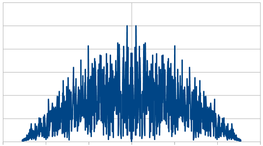
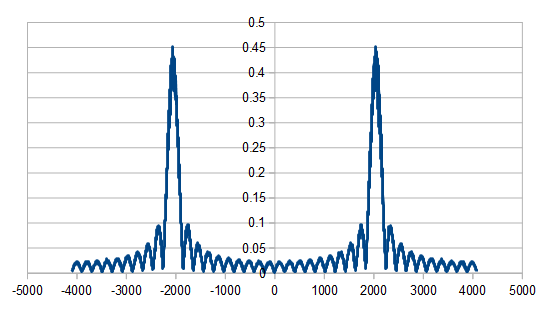
Blue Triangular and Gaussian Noise
Let’s say you roll two dice and subtract one from the other. This is triangular white noise like we saw above.
If you name your dice A and B, you can now reroll A and and take your second number as A-B. You can then reroll B and take B-A as your third number. You then reroll A and take A-B as your fourth number, and so on. This is triangular blue noise!
By only rerolling one of the dice, and flipping which dice is subtracted from the other, you are high pass filtering the white noise and getting blue noise.
In more plain terms, by only re-rolling one of the dice each time, but flipping the sign of the dice, the sum is going to tend to be more different to the last value. That makes for random numbers that have stronger high frequency components.
Here are the results from the program of doing this 16 times:
2, 0, -2, 3, -1, 2, -2, 0, -2, 5, -5, 3, -2, 2, 2, -3
As you can see, the numbers are usually pretty different to the numbers around them, which is different than the white noise case. This is blue noise.
Just like red noise, where you add the dice instead of subtract, this also gives you a triangle distribution, but the triangle is centered on zero. At 8192 rolls, the histogram looks like a wobbly triangle like below, but averaging 100 different runs of 8192 rolls it looks like a perfect triangle (not shown).
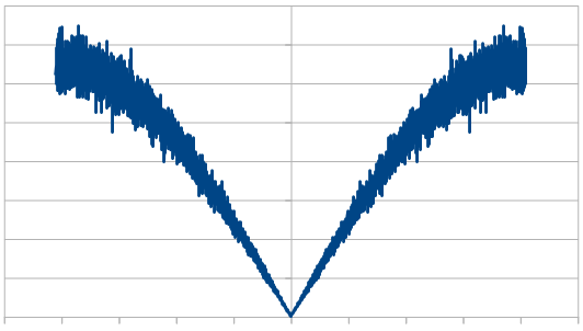
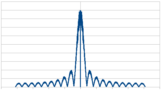
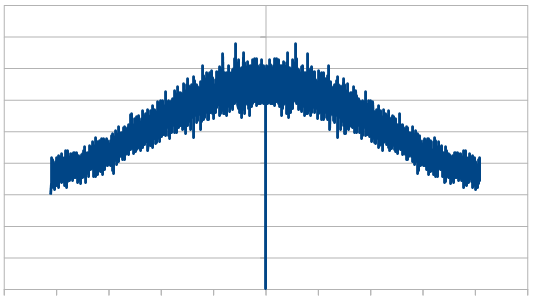
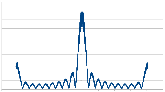
Here it is in frequency space for 16 samples:

Here is 1024:
Here is 8192:
Here is the average of 100 different 8192 runs:

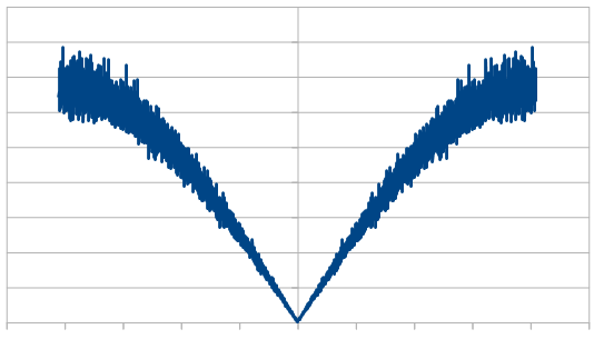
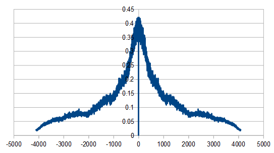
So, the histogram shows a triangular distribution, and the frequency space shows high frequency content. We have triangular blue noise!
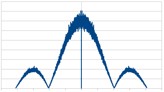
What if we use a different number of dice, like we did for red?
Here’s what we are going to do… we’ll roll N dice to start out, multiply every even numbered die by -1 and sum them up to get our first number. We will then reroll die 0, multiply every odd numbered die by -1 and sum them up to get our second number. We will then reroll die 1, multiply every even numbered die by -1 and sum them up to get our third number. Repeat this process to get as many numbers as you want.
The histogram gets more Gaussian for higher numbers of dice, just like it did for red noise, so I will only show the frequency information for different numbers of dice. All results are the average of 100 different 8192 sequences.
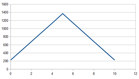
Here it is with 3 dice:
Here it is with 4 dice:
Here it is with 10 dice:
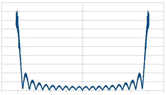
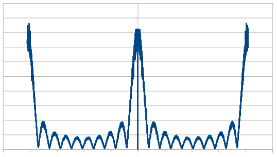
Here it is with 20 dice:

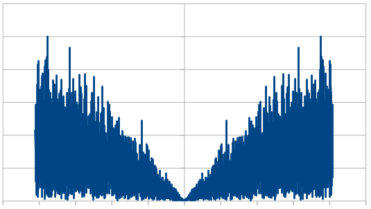
Just like with red noise, for every dice added, we also get “half a hump” in the frequency space. The noise is undeniably blue though, as the largest peaks are on the sides, where the high frequencies are.
If you are curious, here’s 16 rolls of 20 dice being used to make blue noise, which means only re-rolling one dice each roll. Every other number flips sign just about, except near the end where a 3 and a 2 are next to each other.
-9, 9, -7, 7, -5, 7, -6, 5, -6, 6, -3, 3, 2, -3, 3, -2
If you think the numbers are trending toward zero, you are right, but it’s just a short term anomaly. Here are the next 16:
-1, 1, -3, -2, 1, 3, -3, 2, -1, -3, 4, -3, 7, -6, 7, -8
If you wanted the numbers to be strictly positive, or to be within specific values, you could shift (add) and scale them to be in the range you wanted.
All this time, we’ve only been rerolling one die. What if we re-roll a different number of dice, like we looked at with red noise?
Here we roll 20 dice, but reroll 5 each time (cycling through the dice). We did this 8192 times, and averaged the results of doing that 100 times. In frequency space it looks a lot like our 4 dice case. We had that same result with red noise.
Here it is rerolling 10 dice each time, which looks a lot like our 2 dice case.

Here we reroll 15 dice each time.

Here we reroll 19 out of the 20 dice each time, which looks nearly like white noise.
The histogram was unaffected by all of this – at 20 dice it is very Gaussian –
but the frequency make up changed quite a bit. As we rerolled more dice, it started to look more like white noise, which is the same as we saw with the red noise.
I won’t show it, because it’s redundant and there are a lot of images on this post already, but this method of making blue noise also works when sampling from a Gaussian distribution, just like it did with red noise.
If you ever wanted to generate blue rectangular noise, you should look into Mitchell’s best candidate algorithm, using it in 1D. (https://blog.demofox.org/2017/10/20/generating-blue-noise-sample-points-with-mitchells-best-candidate-algorithm/)
You could also look into low discrepancy sequences, which have some similar properties to blue noise (depending on what you are looking for) but are deterministic instead of randomized.
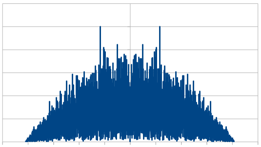
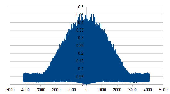
Purple Triangular and Gaussian Noise
What happens if we make blue noise and add red noise to it? Would we get purple noise? Yes we would 😛
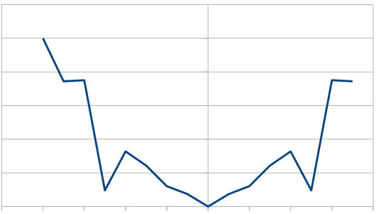
Purple noise is band stop filtered white noise. It has low and high frequency components but doesn’t have much in the way of middle frequency components.
We’ll be doing 20 dice red noise with 1 reroll, and 20 dice blue noise with 1 reroll, and adding them together to get purple noise.
Here are 32 purple noise values made with the process above:
52, 47, 50, 52, 53, 59, 52, 59, 50, 55, 55, 59, 61, 58, 66, 57, 59, 59, 57, 51, 51, 54, 59, 52, 54, 50, 53, 50, 61, 53, 63, 56
Now we’ll do this 8192 times to get that many numbers, and average the result of 100 such runs, to show you the histograms and frequency amplitudes.
Here is the histogram and frequency amplitudes of 16 rolls:


Here is 1024 rolls:


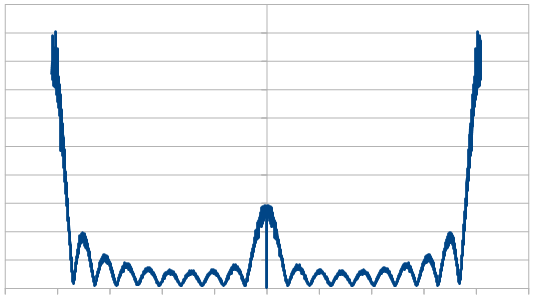
Here is 8192 rolls:

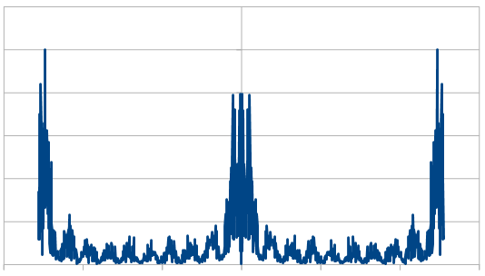
Here is the average of 100 different 8192 rolls:

The histogram is very rough, but does settle into a Gaussian curve like it should. The frequency components show strong low and high frequencies, but not much in the middle.
We could play around with re-rolling different amounts of dice, and different amounts of dice for red vs blue, but I’ll leave that to you if you are curious about it 😛
Purplish Noise
So interestingly, if you generate N blue noise numbers and N red noise numbers, you can lerp between the number sets. Like the first number could be 25% blue and 75% red.
Doing this lets you control how red or how blue the numbers are.
Following are the histograms and DFT magnitude data for red noise made with 20 dice and 1 reroll, lerped towards blue noise made with 20 dice and 1 reroll. These are the average of 100 different 8192 runs.
First, 1% red, 99% blue. There is a strange spike near zero in the histogram I can’t explain, but I don’t think is a bug in the program. If you know what is causing it, let me know!


Next is 25% red, 75% blue.

Next is 50/50, which looks like regular old purple noise.

Here is 75% red, 25% blue.

Lastly here is 99% red, 1% blue.

Before moving on, what happens if we take the max of blue and red noise? This is kind of a throw back to the post that talks about what happens when you take the max of two (uniform white) random numbers. https://blog.demofox.org/2019/06/01/taking-the-max-of-uniform-random-numbers/
Sadly, it just makes red noise with a Gaussian distribution. Nothing special there are far as I can see.
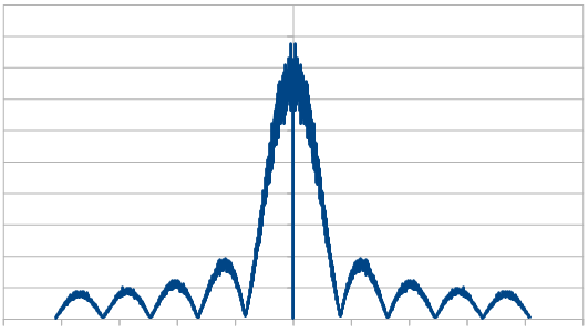
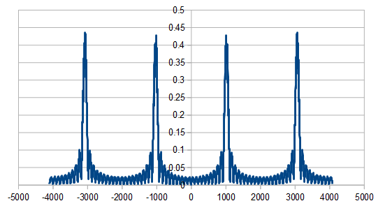
Green Triangular and Gaussian Noise
Green noise is the opposite of purple noise and is band pass filtered white noise. Green noise doesn’t have much high or low frequency to it, but it has middle frequencies.
I wasn’t sure how to generate green noise so asked online to see if anyone knew how or had any ideas.
https://twitter.com/eigenbom (Ben Porter) had an idea of basically mixing blue and red techniques together.
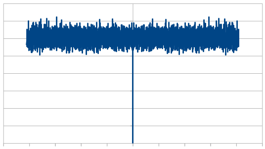
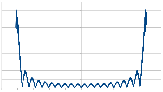
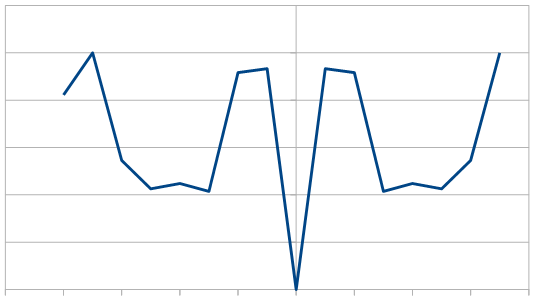
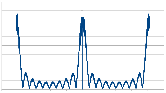
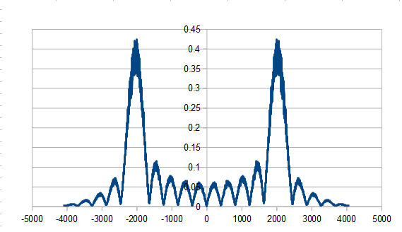
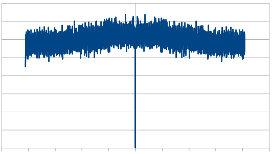
Rolling 20 dice (0 to 5), rerolling one die each roll, and flipping the signs of dice every TWO rolls instead of every roll, you do get a nice green noise as you can see in this DFT below. The histogram was Gaussian.

Trying to generalize this idea, I tried changing the “sign flip period” to other values. That didn’t generalize it very well and I got some strange results. If you are curious, check out the output of the program!
https://twitter.com/thingcreator (@Ray) also had some thoughts on how to generate blue noise, which was more based on some deep DSP ideas.
The first idea is to interleave zeros into blue noise, to decrease the high frequency amplitudes of blue noise to lower frequencies.
Doing that screws with the histogram, since half of the values are zeros, and also screws with the randomness since every other value is zero.
But, it does make some nice green noise!

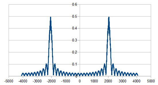
Ray had another idea. Instead of zeros, you could just interleave two independent blue noise streams. This doesn’t screw with the histogram or the randomness like adding zeros does.
I do that by generating blue noise, chopping it in half, and then interleaving the halves. Doing that gives the expected Gaussian histrogram, and still gives a very nice green noise DFT.
What if you do that “chop in half and interleave” multiple times? The histogram will stay the same because the numbers used are all the same, but the frequencies should change.
Here it is being done twice instead of once:
Here it is 3 times:

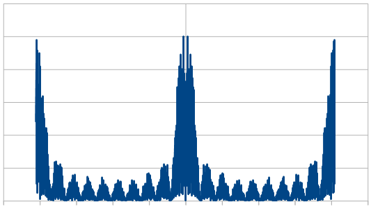
Here it is 10 times:
Here are 32 green noise numbers using Ray’s technique of interleaving two blue noise streams. You can see how it has both rapid change (blue noise qualities) and similar numbers (red noise qualities).
-9, 1, 9, 4, -7, -5, 7, 1, -5, 0, 7, -2, -6, 1, 5, -5, -6, 5, 6, -6, -3, 2, 3, -3, 2, 7, -3, -9, 3, 8, -2, -8
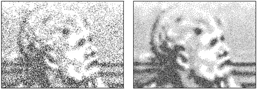
Green noise apparently has some usage in dithering physical objects (like shirt designs). The idea seems to be that green noise is more stable in the physical world without tiny high frequency blue noise features that are more likely to be damaged. https://www.semanticscholar.org/paper/Green-noise-digital-halftoning-Lau-Arce/3e9b673900f86546db94b0922932ce13db84bf75
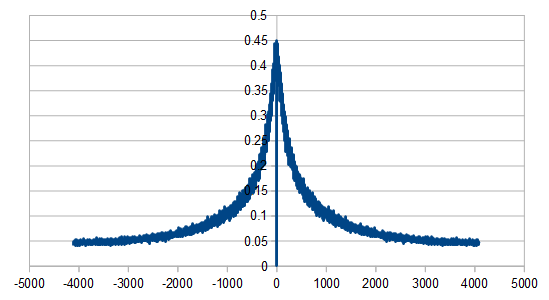
Pink Noise
I’ve known pink noise as “red noise mixed with white noise” for a long while but didn’t think much of it as a noise color. I didn’t know of a usage case for it.
It turns out that pink noise is a pretty important noise color and that many natural and biological processes have this situation where there is some low frequency (red noise) trend over time, but also a small scale randomness (white noise) added on top.
There’s a famous paper by Voss that describes an algorithm to generate pink noise.
You start by rolling some number of dice and adding them up.
From there, you re-roll dice 0 every roll, dice 1 every 2 rolls, dice 2 every 4 rolls, dice 3 every 8 rolls and so on. If you know how to count in binary you should see a pattern emerging.
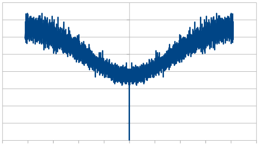
Doing that, the histogram is just Gaussian, but the DFT looks like a bit like a fuzzy red noise, due to the white noise added into the red noise to make pink noise:

Here are 32 pink noise values made with that algorithm:
6, 4, 9, 10, 6, 9, 5, 6, 15, 17, 10, 11, 14, 15, 14, 13, 15, 13, 13, 11, 7, 8, 9, 8, 14, 16, 17, 18, 16, 11, 11, 14
McCartney has a variation on this algorithm where you only reroll one die each roll. The number of leading zeros in your roll number in binary is the number of the dice to reroll. That makes it a more even workload for how many random numbers you generate each time.
It doesn’t affect the histogram, but here is the DFT, which is a little bit sharper in the middle:

Here are 32 pink noise values made with this algorithm:
6, 4, 7, 9, 11, 11, 10, 8, 11, 11, 12, 13, 12, 16, 15, 15, 15, 13, 11, 12, 11, 9, 14, 15, 13, 11, 8, 10, 13, 15, 15, 11
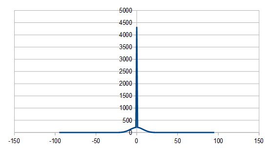
The last variation of the voss algorithm for generating pink noise I’ll show is a stochastic one. It uses a geometric distribution random number each roll to figure out which die to reroll.
This makes for a very sharp frequency spike:
Here are 32 values made with that algorithm:
6, 8, 8, 6, 7, 9, 4, 6, 9, 10, 9, 9, 7, 9, 6, 10, 9, 9, 8, 9, 9, 14, 10, 9, 11, 9, 8, 8, 5, 4, 4, 3
Here is some more info about the voss algorithm
https://www.dsprelated.com/showarticle/908.php
Closing
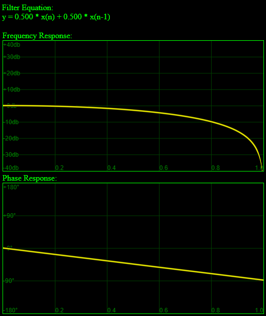
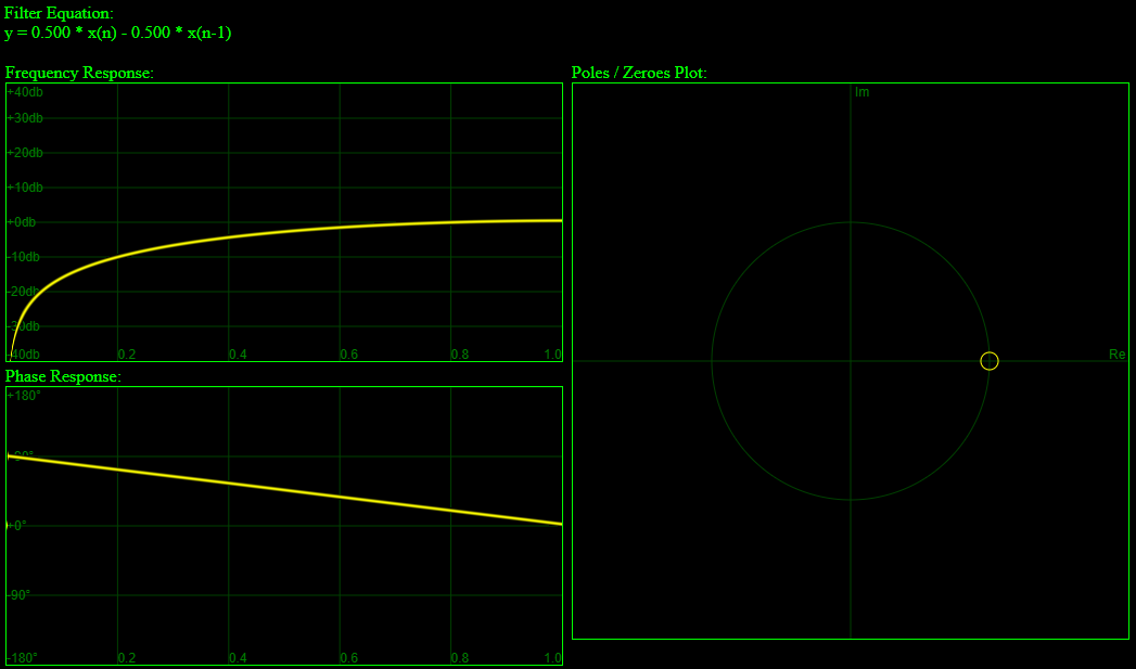
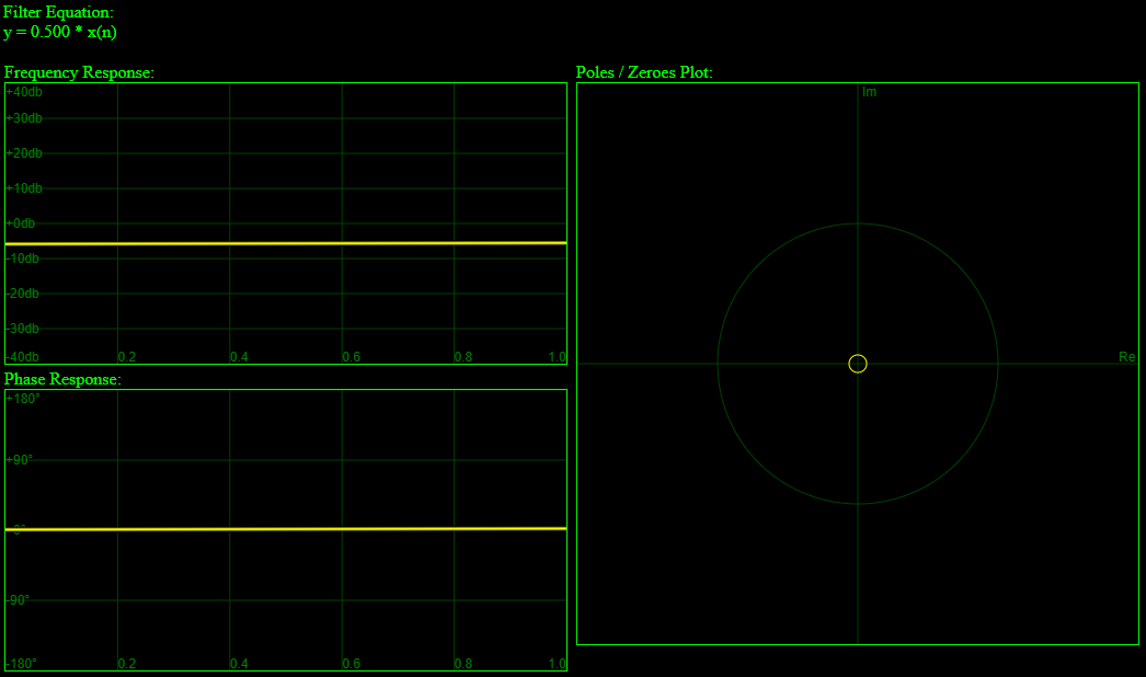
This stuff may seem a bit strange, ad hoc, and magical, but thanks to Ray for pointing this out, this is all just “Finite Impulse Response” DSP stuff. Rerolling dice is like numbers falling out of the delay line, and changing the signs of numbers and summing them (etc) is just filter coefficients for the N order filter used for the N dice.
There’s definitely some deeper DSP stuff here that unifies it all and makes it make a lot more sense that I don’t understand. (yet. Hopefully will one day.)
Here is some interesting info linking this stuff to convolution
https://stats.stackexchange.com/questions/331973/why-is-the-sum-of-two-random-variables-a-convolution/331983#331983


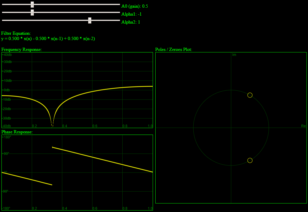
 is the filtered sample,
  is the current unfiltered sample,
  is the previous unfiltered sample, and
  and
and  are values to multiply the samples by to control the filtering.


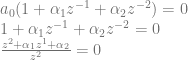
 with
with  to get this equation:


 , which will let us plug in different frequency values for omega (
 ) to see how the filter affects those frequencies.
 . Another way to write that is
  . That shows that we can multiply any point in our complex sinusoid signal by
  to get the previous sample, which is super handy, as it delays the signal by one sample.

 .
.
 divided by
 , which makes our transfer function look like the below.

 which also controls how the frequencies are filtered. You can also multiply
  value for use in the difference equation.

 :
:


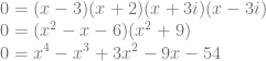
 . In our case, x is z, A is 1, B is


 . So, if


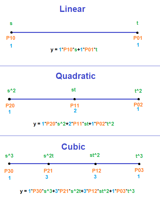
 , like in the linear Bezier curve formula below (which is also just a lerp):
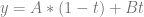
 and
and  . That lets us write the same equation like the below:

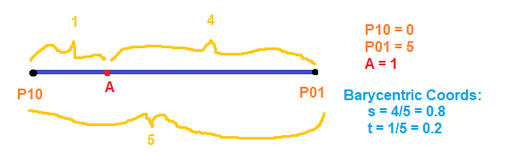


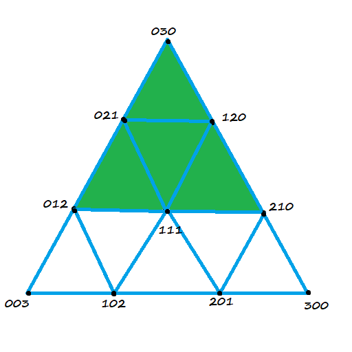
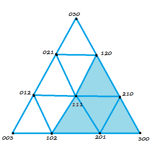
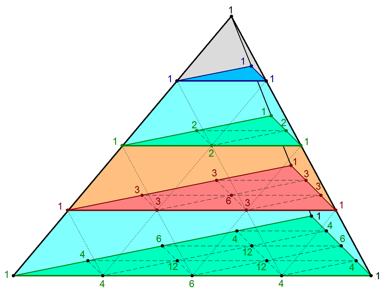
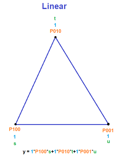
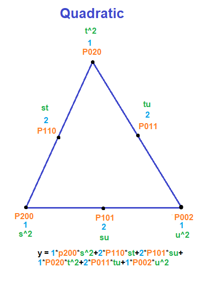
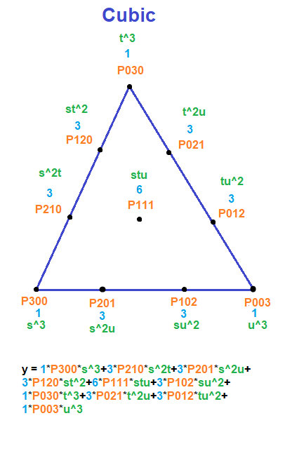
 . If we want to make a degree N curve, our control points will be all the x,y pairs that add up to N. Here are the control points for the first few degrees of Bezier curves.
 ,
, 
 ,
,  ,
, 
 ,
,  ,
,  ,
, 
 ,
,  ,
, 
 ,
,  ,
,  ,
,  ,
,  ,
, 
 ,
,  ,
,  ,
,  ,
,  ,
,  ,
,  ,
,  ,
,  ,
, 


 .
. .
. and this is called the joint probability.
 and it means “What is the probability of A happening, if B has happened?”