
There’s an interactive Bezier Triangles webGL demo I made that goes with this post, and what i used to make the 3d rendered images with. You can find here:
http://demofox.org/BezierTriangle.html

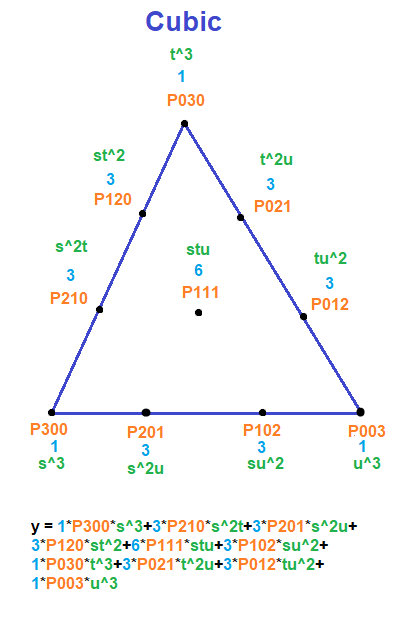
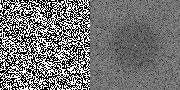
Above is a cubic bezier triangle which has 10 control points. Each edge of the triangle is a cubic Bezier. That makes for 9 control points, and the 10th control point is in the center of the triangle.
I’ve been thinking more about using raytracing for data lookups (https://blog.demofox.org/2018/11/16/how-to-data-lookups-via-raytracing/) and have been trying to think of how you might get higher order interpolation than linear barycentric interpolation. The hope is to fit the data better, and with fewer data points, resulting in a sparser data mesh.
The higher order interpolation may take a little more compute and memory access, but having fewer triangles to raytrace against is a good thing (smaller BVH) besides the potentially better data fit. There’s a trade off here, I’m sure – and I’m sure that trade off is situational.
In the past, I found a way to exploit the linear interpolation of texture samplers to get higher order interpolation (https://blog.demofox.org/2016/02/22/gpu-texture-sampler-bezier-curve-evaluation/) but when thinking about how to extend that to triangles in a vertex shader, I never found a good way to do it.
One of the challenges in the vertex shader triangle case is not easily being able to get barycentric coordinates on the triangle, but that’s drop dead simple in the raytracing case, since barycentric coordinates are one of the few pieces of data you actually have out of the box.
These ideas came together and I realized it was time to finally dig into the guts of Bezier triangles.
Luckily, it turns out they are not that scary!
Here is some info on Bezier curves that are good background for the rest of this post:
- One Dimensional Bezier Curves: https://blog.demofox.org/2014/08/28/one-dimensional-bezier-curves/
- The De Casteljau algorithm for Evaluating Bezier Curves: https://blog.demofox.org/2015/07/05/the-de-casteljeau-algorithm-for-evaluating-bezier-curves/
- Rectangular Bezier Patches: https://blog.demofox.org/2015/07/28/rectangular-bezier-patches/
Bezier Simplex and Barycentric Interpolation
Bezier triangles are very close conceptually to Bezier curves, and in fact, both of them are examples of a Bezier Simplex.
A simplex is the shape with the fewest number of points to create an object in a given dimension.
A 0 dimensional simplex is a point, a 1 dimensional simplex is a line, a 2 dimension simplex is a triangle, a 3 dimensional simplex is a tetrahedron, and so on.
Barycentric coordinates are coordinates on a simplex, and sum up to 1.0.
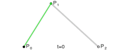
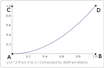
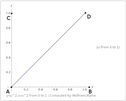
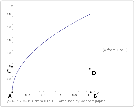
Bezier curves are parameterized by a value 
Another way to think of this though is that there are two parameters 


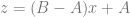
That is 1 dimensional linear barycentric interpolation between the values A and B on a line.
We can bring that up to 2 dimensions to get a linear barycentric interpolation between 3 points on a triangle.

That extends to any dimension by just adding more terms.
Much like we can bring this concept to higher order interpolation on a line with Bezier curves, we can do higher order Barycentric interpolation on simplices of higher dimensions. If you do this with a triangle, you get a Bezier triangle. If you do this with a tetrahedron, you get a Bezier tetrahedron, and so on.
Calculating Barycentric Coordinates
Calculating the barycentric coordinates is conceptually pretty simple.
- Start with an N dimensional simplex.
- When you place a point in it, that divides the simplex into several simplices of the same dimension. Each of these other simplices will be opposite a point on the larger simplex.
- Calculate the area of a smaller simplex and divide it by the area of the large simplex. This is the barycentric coordinate of the point that is opposite this simplex.
That explanation might have been a little thick. Lets look at lines and triangles as an example.
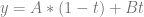
First is lines:
The point A divides the line (1-simplex) into two parts: P10 to A, and A to P01. P10 to A is 1 unit long. A to P01 is 4 units long. The entire line’s length is 5 units long.
To calculate the barycentric coordinates (s,t) we first start with s.
The simplex opposite P10 is the A to P01 line segment, which has a length of 4. Dividing that by 5, we get a value of 0.8. So, the value of s is 0.8.
The value of t can be found the same way. The opposite line segment of P01 is P10 to A and has a length of 1, which we can divide by 5 to get 0.2. We could have also just calculated 1 – 0.8 since they have to add up to 1.0!
The Barycentric coordinates of point A on that line is (0.8, 0.2).
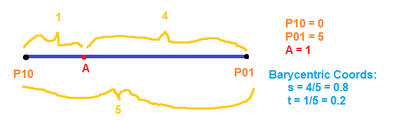
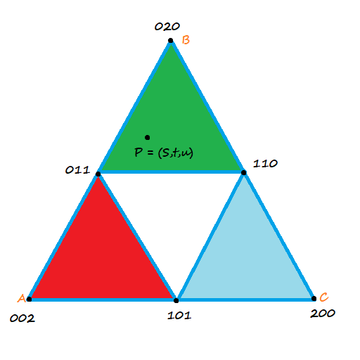
Calculating the Barycentric coordinates of a triangle is very similar. In the image below, point A has Barycentric coordinates of (0.5, 0.333, 0.166)
A point is known to be inside a simplex if all the components of it’s Barycentric coordinates are between 0 and 1.
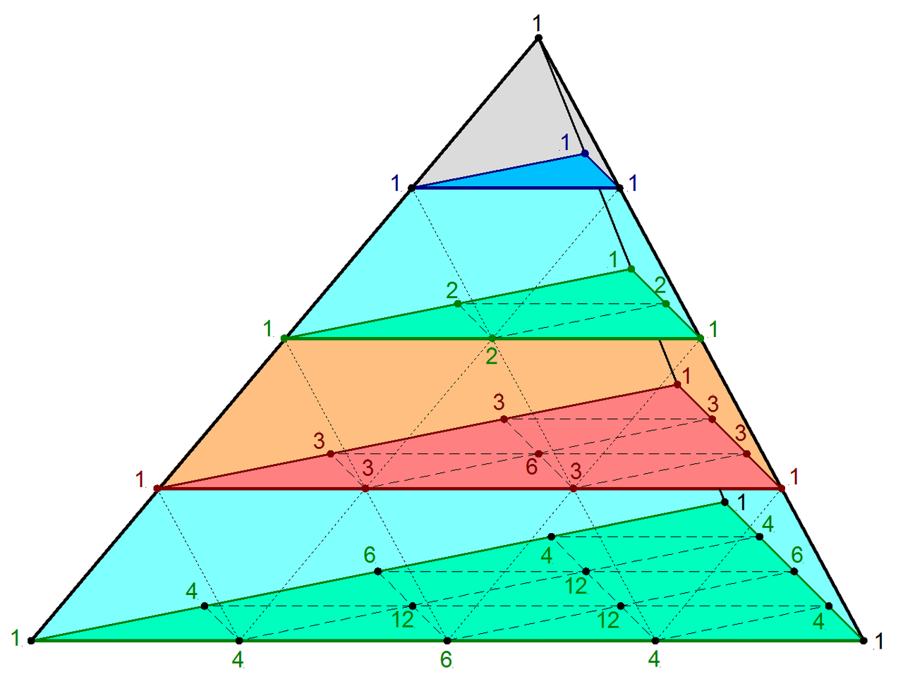
The De Casteljau Algorithm For Bezier Triangles
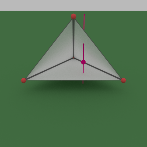
Starting with linear Bezier triangles, you have a control point at each corner of the triangle, and you use barycentric interpolation of those values to get the value at a point on the triangle.
This is a linear interpolation (the result is on a plane), and is what we’ve been doing in vertex shaders since vertex shaders existed. Simple barycentric interpolation.
Much like how a linear Bezier curve is a linear interpolation (lerp) between two values, a linear Bezier triangle is a linear interpolation between three values. Each edge of the triangle is also a linear Bezier curve.
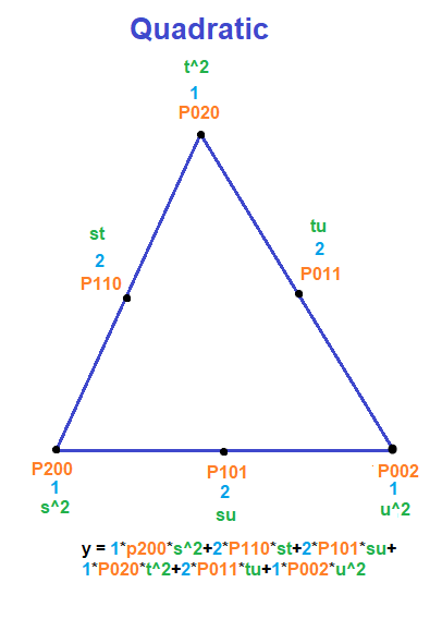
Next up is a quadratic Bezier triangle.
A quadratic Bezier curve is made by linearly interpolating between two linear Bezier curves. A quadratic Bezier triangle is made by linearly interpolating between three linear Bezier triangles.
Here is a refresher on how a quadratic Bezier curve actually works. There are 3 control points A, B, C. One linear interpolation is from A to B. The other linear interpolation is from B to C. These values are linearly interpolated for the final point on the curve.
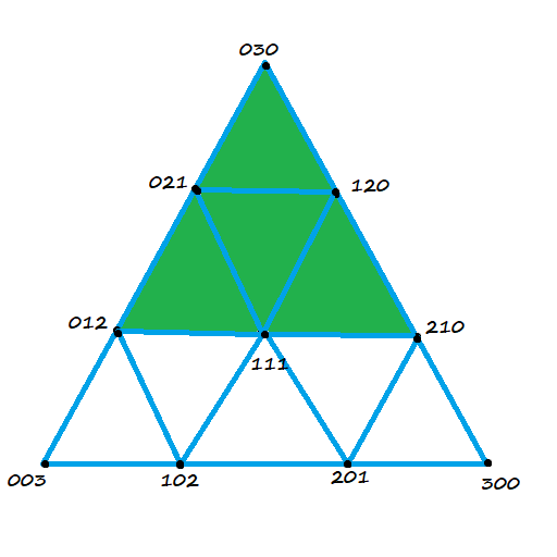
How does this work on a Bezier triangle? Each edge of the triangle in a quadratic Bezier curve which gives us control points like the below:
What we do first is use point P’s Barycentric coordinates to interpolate the values of the red triangle: 002, 011, 101 to get point A. You treat those values as if they are at the corners of the larger triangle (if you think about it, this is how quadratic Bezier curves work too with the time parameter. Each line segment has t=0 at the start and t=1 at the end).
We next interpolate the values of the green triangle: 011, 020, 110 to get point B.
We then interpolate the values of the blue triangle: 101, 110, 200 to get the point C.
Now we can do a regular linear barycentric interpolation between those three values, using the same barycentric coordinates, and get a quadratic Bezier triangle. Each edge of the triangle is also a quadratic Bezier Curve.

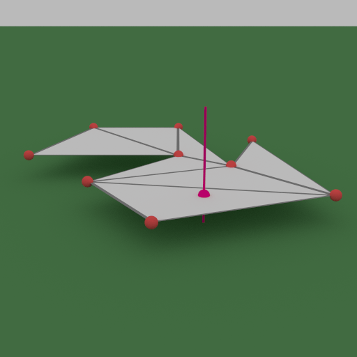
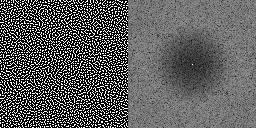
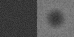
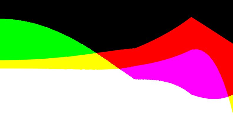
For a cubic Bezier triangle, it’s much the same. You evaluate a quadratic Bezier for each corner, and then linearly interpolate between them to get a cubic. Below is an image showing the control points used to create the three quadratic Bezier triangles.

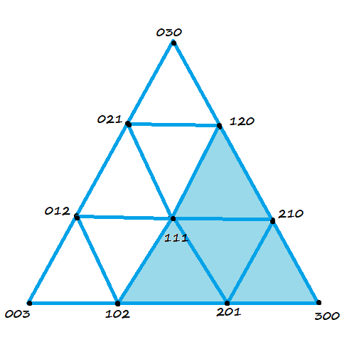
Which results in a cubic Bezier triangle. The edges of this triangle are cubic Bezier curves.
This works the same way with any Bezier simplex by the way.
The Formula For Bezier Curves
Just like Bezier curves, you can come up with a multivariable polynomial to plug values into for Bezier Triangles, instead of using the De Casteljau algorithm. The De casteljau algorithm is more numerically stable, but the polynomial form is a lot more direct to calculate.
Let’s consider Bezier curves again first.
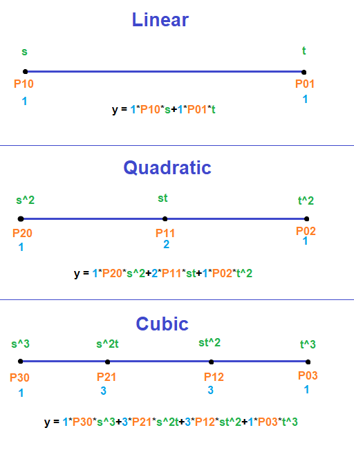
Lines (a 1-simplex) have two points, so we’ll describe control points as 
- Linear:
,
- Quadratic:
,
,
- Cubic:
,
,
,


You might notice that a degree N curve has N+1 control points. Linear curves have 2 control points, quadratic curves have 3 control points, cubic curves have 4 control points and so on.
The index values on these control points tell you where they are on the line, and they also tell you the power of each barycentric coordinate they have, which we will get to in a minute.
The last part of making the formula is that the control point terms are also multiplied by the Nth row of Pascal’s triangle where row 0 is at the top row. (Pascal’s triangle image from https://brilliant.org/wiki/pascals-triangle/)
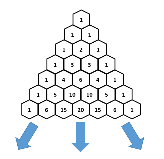
Doing that, you have everything you need to create the familiar Bernstein basis polynomial form of Bezier curves.
The image below puts it all together. Orange is the name of the control point, which you can see also describes where it is on a line. The index values of the control point also describe the power of the Barycentric coordinates s and t which are in green. Lastly, the row of pascal’s triangle is in blue. To get the formula, you multiply each of those three things for each control point, and sum them up.
The Formula For Bezier Triangles
You can follow the same steps as the above for making the formula for Bezier triangles, but you need to use Pascal’s pyramid (aka trinomial coefficients) instead of Pascal’s triangle for the control points. (image from https://en.wikipedia.org/wiki/Pascal%27s_pyramid)
This time, we have 3 index numbers on control points instead of the 2 that curves had, but we still find all permutations which add up to N.
Here are the control points for the first few degrees of Bezier triangles.
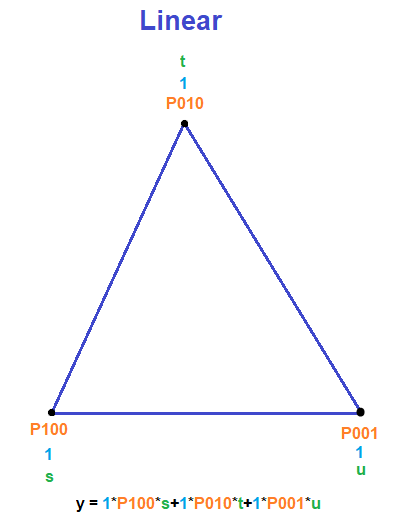
- Linear:
,
,
- Quadratic:
,
,
,
,
,
- Cubic:
,
,
,
,
,
,
,
,
,


Below are diagrams in the same style as the last section, which show the equation for a Bezier triangle and how to come up with it.
This pattern works for any Bezier simplex.
Use For Data Lookup On the GPU
If you wanted to use this for data lookup, you’d first have to fit your data with a Bezier triangle mesh, using whatever degree you wanted to use (quadratic or cubic are the seemingly likely choices!). The fit would involve not only finding the right values to give at control points, but also the right location to put the vertices of the triangles, so that you could make the mesh sparser where you could get away with it, and denser where you needed it.
Doing that fit sounds challenging, but I bet doing gradient descent of vertex positions and control points could be a decent place to start. Simulated annealing probably would help too.
Once you have your data fit, you need to figure out how you are storing it. Linear Bezier triangles only need data stored per vertex, but quadratic ones store data per edges too, and cubic ones store data per triangle. Beyond cubic, no special class of storage is needed.
Storing data per vertex and per triangle is easy, because that’s the paradigm we work with already in graphics (and raytracing specifically). The per edge data is harder. The reason that it’s harder is that to be fast, you want it to be a simple array, where you index it by the two neighboring triangles of the edge. A 16 bit index for triangle A and 16 bit index for triangle B means a 32 bit index into the edge data array. The problem is, that data is extremely sparse (each triangle index will connect to just 3 other triangle indices. The rest of the entries will be empty / useless!), so making a simple array is a lot of wasted space, and frankly is just a lot of space in general.
One idea is to store edge information in the per triangle data, even though it’s redundant (neighboring triangles would have duplicate info for the shared edge). It still would be a simple lookup.
Another idea is to store 3 edge indices in each triangle and use that to look up into an edge array for the per edge data. The memory usage here is minimized to only what is needed, but it’s a double dereference, so is pointer chasing on the GPU which doesn’t sound very nice.
Another idea would be to use minimal perfect hashing (https://blog.demofox.org/2015/12/14/o1-data-lookups-with-minimal-perfect-hashing/). What that would allow you to do is get a hash function where you could put in the triangle index and which edge you were querying for (0, 1 or 2) it would give you as output the index into an edge array to get the data from. This is different from the last one because you aren’t reading an index for the edge, so is one less dependent data lookup.
Once you have your mesh fit, and you have a way to look up the data needed to evaluate a point on your Bezier mesh, assuming your mesh is oriented on the X,Z plane, with a Y value of 0 (the “height” data being stored in a different data channel), you can shoot a ray from (x,y,1) to (x,y,-1) for the (x,y) point you want to do a data lookup for. The ray will hit a triangle, give you barycentric coordinates, the triangle id, and enough info for you to read the control points for that triangle.
From there, you do your calculations and get your result. All done!
Is This a “1D” Bezier Triangle?
You might have noticed that with things as I’ve described them, control points can only be moved up and down on the vertical axis, but not on the horizontal plane.
That is true and this is a simpler form of a more general Bezier triangle.
If you want control points that you can move in any direction in 3d, all you need to do is make one Bezier triangle that you evaluate to get an X axis value, another to get a Y axis value, and another to get a X axis value.
Using it for data lookup seems to go out the window, but for other usage cases, this is probably useful knowledge.
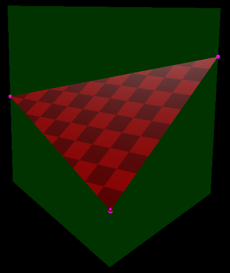
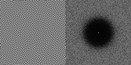
How Did You Render The Surfaces?
TL;DR I use ray marching, but keep reading for more details.
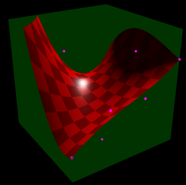
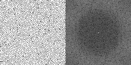
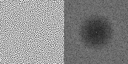
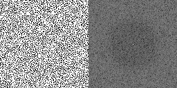
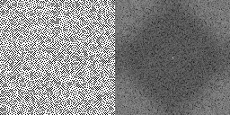
How the 3d surfaces were rendered (the red/black checkerboard 3d images) is nearly out of scope of this post, but someone asked so I thought I’d share. Feel free to “view source” on that demo. It’s written in webgl so should be pretty easy to follow the shader etc.
First, i get a ray starting position and direction for each pixel of the image.
I next intersect that ray against a triangular prism shape (the green background you see behind the object). I do that by intersecting the ray by each plane that makes up that shape, and keeping track of the min and max hit time of the ray. If the min > the max, i know the ray missed the bounding shape and i can just draw black.
Next up, I calculate if the min time of the intersection is above or below the triangle bezier surface. I do this by getting the (X,Y,Z) position of the ray at that time, using (X,Z) to calculate Barycentric coordinates, using those to evaluate the triangle and see if the triangle’s height at that point is above or below the ray’s height (Y axis value).
Next, i take up to 20 steps from the start time to the end time, stopping when either the “aboveness” of the ray changes (meaning it intersected the surface) or if i get to the end of the 20 steps and nothing was hit.
If the ray intersected the surface, i check how much above the surface the ray was on the previous step vs where it is in the current step, treat it as a line (make a y=mx+b function out of these data points!) and solve for zero. I take that as my intersection point.
I next calculate the gradient of the surface using finite differences (https://blog.demofox.org/2015/08/02/finite-differences/), forward differences specifically, and use that to get a surface normal for shading.
Some improvements that could be done here…
- It’s possible to get the gradient of a Barycentric triangle analytically, and isn’t that difficult since it’s just a polynomial. Doing that instead of finite differences would make a more accurate and better gradient.
- Instead of taking 20 fixed sized steps, I could use the gradient to get a distance estimate to be able to take larger steps down the ray when it’s farther from the surface (more info here: https://iquilezles.org/www/articles/distance/distance.htm)
- If this needed to run faster, the step count could be dropped down to a smaller number. If you did that though, you’d start to notice “stairs” and other artifacts. A way to combat these visual problems would be to use a screen space blue noise texture as a “random number” from 0 to 1 to push each ray down that percentage of a step away from it’s starting point. That would turn the visual artifacts into a more pleasant blue noise pattern – the error would be evenly distributed and be much harder to notice. If you animated that noise well over time, it would look even better. If you did this under TAA, and possibly switched to interleaved gradient noise (something to try, not a slam dunk for sure always better thing IMO), it would look very nice. (more info on animating noise over time https://blog.demofox.org/2017/10/31/animating-noise-for-integration-over-time/ and also the follow up post)
- Another thing to try would be to not do evenly spaced sampling down the ray from min to max time. Uniform sampling is not great. For best results, you’d want to distribute the sampling locations in a 1d blue noise pattern so that it evenly distributed the error and had low aliasing to give you the most pleasant result. This would be hard to be compatible with some of the other options, but is a nice thing to try if not doing them.
Extensions
There are lots of extensions that you could do to these Bezier triangles.
One extension would be to bring this to volumetric data with Bezier tetrahedrons. The result when using it for data meshes would be a tetrahedral mesh. To do a look up for a specific (x,y,z), you would shoot a ray from that point in any direction. The triangle you hit would contain 3 of the 4 points of the tetrahedron. You could shoot a ray in the opposite direction to get another triangle which had the 4th, or you could have data stored for that triangle index which says “if you hit this triangle from the front, the fourth vertex is M, if you hit this triangle from the back, the fourth vertex is N”, which means you just need to do a dot product of the ray and the triangle normal to figure out the fourth vertex, instead of doing another ray intersection against the BVH.
An easy but powerful extension would be that you could calculate the value of a point in two different Bezier triangles and divide the values. This would give you a rational surface which can represent a LOT more shapes than an integral surface can. For example, a quadratic Bezier curve can’t make conic sections (circles, etc), but a rational quadratic Bezier can make them, exactly.
Making it rational is just the R in NURBS, so other extension ideas are… NU = non uniform control points. R = rational instead of integral. BS = B-Spline.
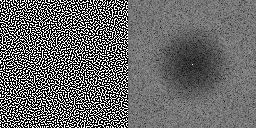
Another extension that you could do is not limit the shape to being inside the simplex. For instance, here’s a cubic Bezier triangle where i let the equations go outside of the triangle, but am still limiting it to a cube. The math is totally fine with this. No division by zeros or any other badness.
Lastly, it turns out you can extend the concept of Barycentric coordinates to convex shapes that aren’t a simplex, such as a pentagon, or a dodecahedron. In the case of a quadratic Bezier pentagon, you would evaluate 5 linear pentagons – one for each corner of the pentagon – and then combine those with another linear Bezier pentagon interpolation. I’m not sure when this would be useful, but it’s definitely possible.
Check out this link for more info about generalized Barycentric coordinates:
https://en.wikipedia.org/wiki/Barycentric_coordinate_system#Generalized_barycentric_coordinates
Links
There are a lot of links in this post, but I found this page to be really helpful for understanding some of the details of Bezier triangles.
https://plot.ly/python/v3/ipython-notebooks/bezier-triangular-patches/


 , alpha works like the below, where
  clamps values to be between 0 and 1:
 .
.
 function changed to encompass the whole second term, instead of just SrcColor! That gives this result that matches the one we got when we did the lerp in shader code:


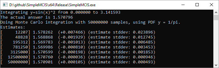
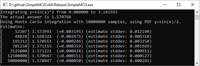
 and you want to know what the area is under the curve between 0 and pi.
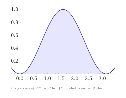
 ), but let’s pretend like we can’t, or don’t want to solve it that way.
 . When we divide by that, it means we end up just multiplying by pi, so it’s mathematically equivalent to what were were doing before!
 . You can see it compared to the function we are integrating
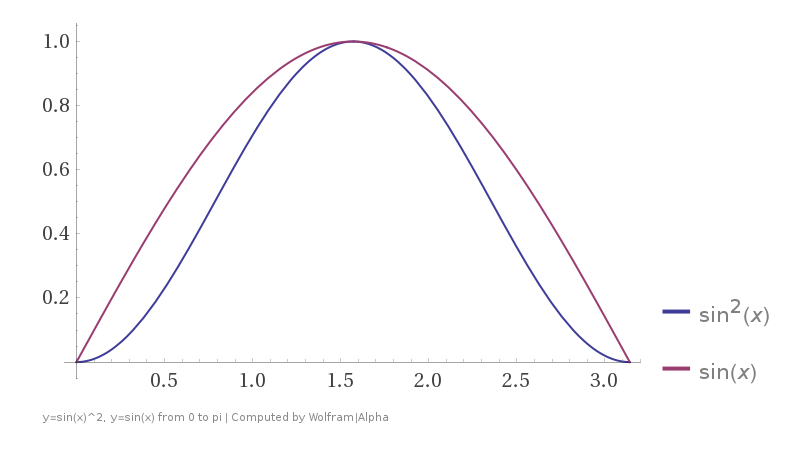
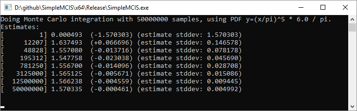
 that is between 0 and 1 and plug it into this function, which is the inverse CDF:
 , which doesn’t look much like the function we are trying to integrate at all:
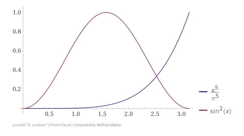


 from the lighting calculations, because the random number distribution handles it for you.
 and solve for y to get
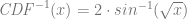
  , but if you try to solve
  for y, you are going to have a bad day!
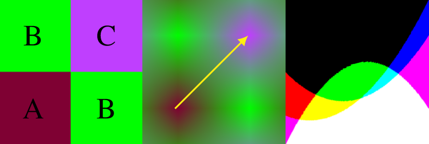
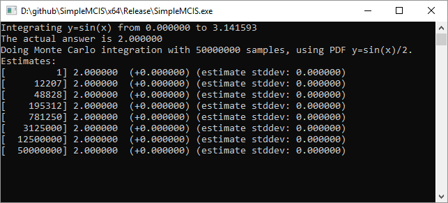
 ?
?

 let’s literally replace
  with
with  and see what we get out.

 and
and  and see what happens for different types of lines.
 .
.

 . This graph shows where that is sampling from on the bilinear surface:

 ,
,  ,
,  .
. . Here’s the graph of where we are sampling on the bilinear surface:

 that goes from 0 to 1. Then we can make


 in for y and see what we get out.


 , which takes this path on the bilinear surface:

 . It scales and shifts the y values to be between 0 and 1.


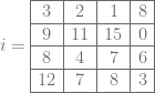
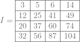

 is the sum of all the values in the rectangle from
  to
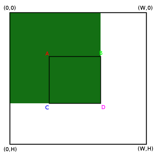
to  inclusively, but what if we want to find the sum of a different rectangle? What if we have 4 points A,B,C,D and we want to know the sum of the numbers within that sub-rectangle?
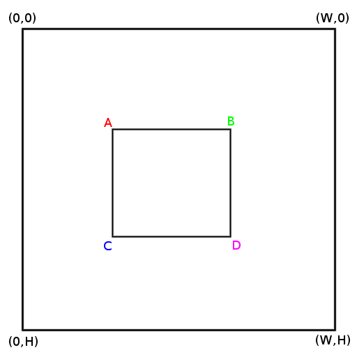


 more bits of storage which means we would need 2 more bits of storage in this case for the 2×2 grid (4 samples), making it be 5 bits total per value (3 bits of storage + 2 extra bits to hold the sum of 4 values). That would let us store the proper table:
 is 0.
is 0. is 2.
is 2.