UPDATE 6/25/2020: The bottom of the post now has a section about using 2D low discrepancy sequences with an alias table and compares results vs the 1D methods. The code has been updated as well to include that stuff.

In this post we are going to talk about Round Robin first, then Weighted Round Robin.

The ~500 lines of standalone C++ that generated the data for this blog post can be found at https://github.com/Atrix256/WeightedRR

Round Robin

Let’s say you find yourself in one of these 2 equivalent scenarios:

1. You want to repeatedly choose from a list of 10 objects in a fair way, where the objects are chosen at roughly the same rate – like, a loot drop table for killing monsters in a game.
2. You have 10 queues of work that you want to process work items from in a fair way, where work is consumed from the queues at roughly the same rate.

In either case you want a stream of integers between 0 and 9 where ideally any section – large or small – should have roughly even counts of those numbers chosen. In other words, it should have a flat histogram for both large and small sections.

One way to deal with this is to just walk through the numbers 0 through 9 over and over and over. You could increment a number whenever you wanted the next index and use modulus to ensure it was between 0 and 9.

I’m calling this “Sequential” in the graphs and that would work, but depending on your usage case, it might be undesirable that it was so obviously going in order from 0 to 9.

Another way to deal with this would be to roll a random integer 0 through 9 and use that as your answer. In the code, I roll a random float between 0 and 1 and remap that to an integer 0 through 9 so it’s more like the other methods. I’m calling this “White Noise” in the graphs and that also would work in that the histogram is going to be flat after an infinite number of samples, but it won’t be very flat in small numbers of samples.

Yet another way to deal with this is to use a low discrepancy sequence (deterministic or randomized aka blue noise) such as the golden ratio additive recurrence low discrepancy sequence which looks like this:

float GetNextValue(float x)
{
  float newX = x + 1.61803398875f;
  return newX - floor(newX);
}

In the above, the first value you ever plug into this function can be any number. It can be 0.0, but it doesn’t have to be.

1.61803398875 is the golden ratio and since we are dealing with values between 0 and 1, you could also use 0.61803398875 instead which is the fractional part of the golden ratio, but is also 1 divided by the golden ratio (the golden ratio conjugate).

The golden ratio is a good choice here because it’s an irrational number, meaning that from a mathematical point of view (ignoring limitations of computers for a second) it won’t ever repeat values.

The golden ratio is also an excellent choice among irrational numbers because it is the most irrational number. Less irrational numbers – like pi – still don’t repeat but they have “near repeats” which make them less good of a choice. Then there are numbers like the square root of 2, which are pretty decently irrational – more than pi, but less than the golden ratio.

An alternate way to write the code is like this, which gives you “random access” to the sequence, but is more prone to having floating point precision issues.

float GetValue(int index, float seed)
{
  float newX = seed + float(index) * 1.61803398875f;
  return newX - floor(newX);
}

If you use this in our problem for generating floating point values between 0 and 1 and remapping to integers 0 through 9, you will get fairly even counts of occurrences of those integers (a fairly flat histogram) from both small and large sections of the sequence.

Here is a screenshot of the program generating a sequence of 80 items, using the techniques talked about so far.

It’s hard to tell what the histogram looks like from that, but it is still a bit interesting looking at the difference in patterns of the numbers chosen. There are seeming patterns even in the golden ratio because the values are quantized to 10 possible values.

Here are histograms of 100 samples. It shows that white noise is doing noticeably worse than the irrational numbers, but the irrational numbers don’t have a winner that is easy to discern with the naked eye. Sequential can’t even be seen because it is by definition a completely flat histogram and so is a flat line at y=0.1.

Here are histograms of 10,000 samples. White noise and pi look about the same, but golden ratio and square root of 2 are much closer to the actual flat histogram value / sequential sequence.

Here are histograms of 1,000,000 samples. White noise is way worse than everything else, but it’s hard to see a winner from the rest of the group.

Here we remove white noise from the graph to see the others better. Pi shows being the worst. Square root of two is next, and then the golden ratio which is closest to the sequential / flat histogram line.

Round Robin vs Random Integers

When using white noise, round robin is just random integers. It’s the same as rolling dice. So what is the difference?

In the last section I say that using a low discrepancy sequence is better than using white noise, because it reaches the target histogram more accurately with fewer samples – fewer rolls of the dice.

The downside to this though is that the numbers are no longer random… a person viewing the sequence of numbers can almost certainly guess what the next number is going to be.

So, that makes it not useful to use these for places where randomization is important – like when gambling or for cryptography.

But, where this is useful is for places where fairness matters but randomness does not.

One example could be pulling work items from a work queue. Who cares if it is possible to guess which thread is going to get assigned the next item of work? The important thing is that the work is spread evenly.

Another example is in numerical integration in monte carlo integration, and also other stochastic rendering situations. This is more what I care about. In these situations, you don’t care if the choice can be predicted or not, but if you can reduce the amount of error vs the target distribution in fewer samples that means you’ll have less noise in your resulting image, which is ::chef kiss:: oh so great. A better image for the same processing power.

If you were in a situation that wanted randomness, but you still wanted some of these benefits, you should check out “blue noise”, which is a randomized version of low discrepancy sequences. A good place to start might be my post on generating blue noise in 2 dimensions, which you could modify to only generate 1 dimensional blue noise and use for this purpose.

https://blog.demofox.org/2017/10/20/generating-blue-noise-sample-points-with-mitchells-best-candidate-algorithm/

Weighted Round Robin

Let’s say you find yourself in the same situation as before but now there are weighted probabilities involved.

• For the loot drop situation, different loot should be awarded with different probabilities.
• For the work queues, you could have different powered CPUs servicing the work queues maybe. More powerful processors should be more likely to get work served to them perhaps.

For our situation, we’ll say that the weight of item 0 is 1, the weight of item 1 is 2, and so on, up to the weight of item 9 being 10.

Let’s check out our options again.

First, we could go sequentially. This means that our sequence would go like this: 011222333344444… etc.

A possible issue with this (again, depending on your specific needs) is that it is even, but it goes through every occurrence of a number before moving to the next number. If it was desired that the numbers be visited in a more interleaved fashion, you’d want to try something else.

The next thing you could try is to take the item weights and divide them by the total of the item weights, so that they add up to 1.0. This would make them normalized. From here, we could roll a random floating point number between 0 and 1, find the item that has the range that contains that floating point number, and use that as the selected item.

That would solve the problem I mentioned, but would introduce the problem of white noise: while large sample counts have the right histogram (distribution), small sample counts don’t.

We could also use irrational numbers again, which would do better at reaching the correct histogram than white noise but become deterministic like sequential, but still shuffled “a bit”.

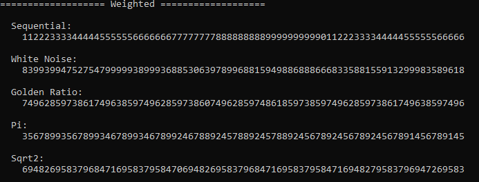
Here’s the program output for 80 item sequences of the various techniques:

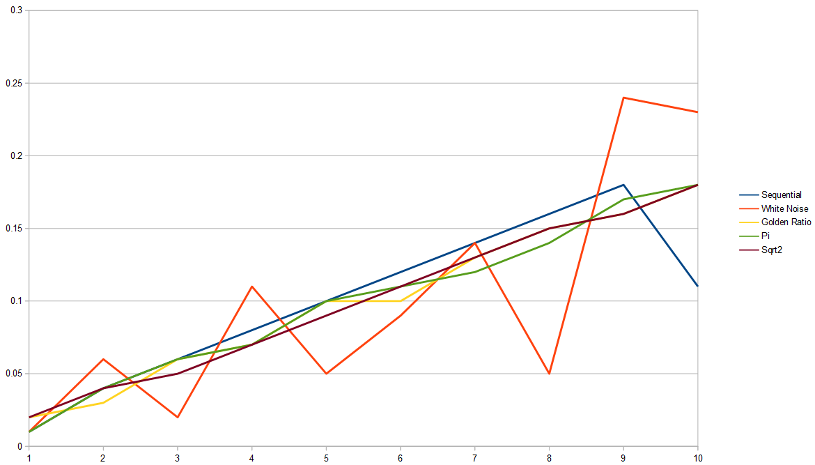
Here are histograms with 100 samples. The irrationals are all doing pretty well. White noise is not doing great. Strangely, sequential is also not doing real great for the last value because the sequence length doesn’t divide 100 evenly this time!

Here are histograms with 10,000 samples. It’s harder to see for sure who is winning by nature of the graph, compared to the last section, but we can see white noise is not doing great.

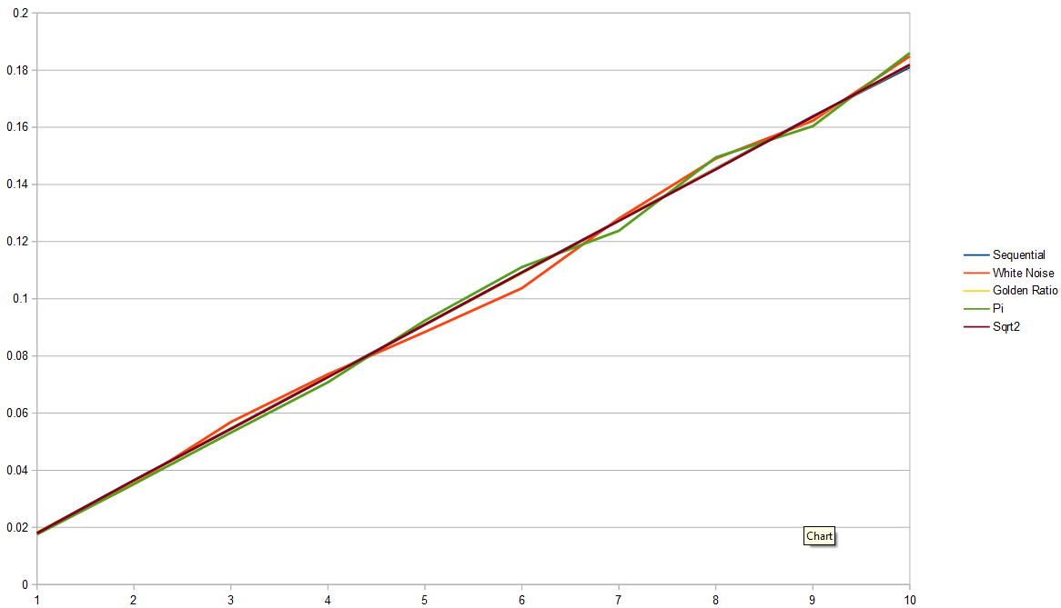
Here are histograms with 1,000,000 samples. It’s nearly impossible to see anything about it.

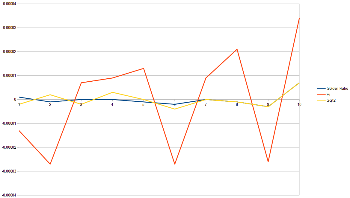
Here is the graph of subtracting sequential from the others. It shows that white noise is by far the worst.

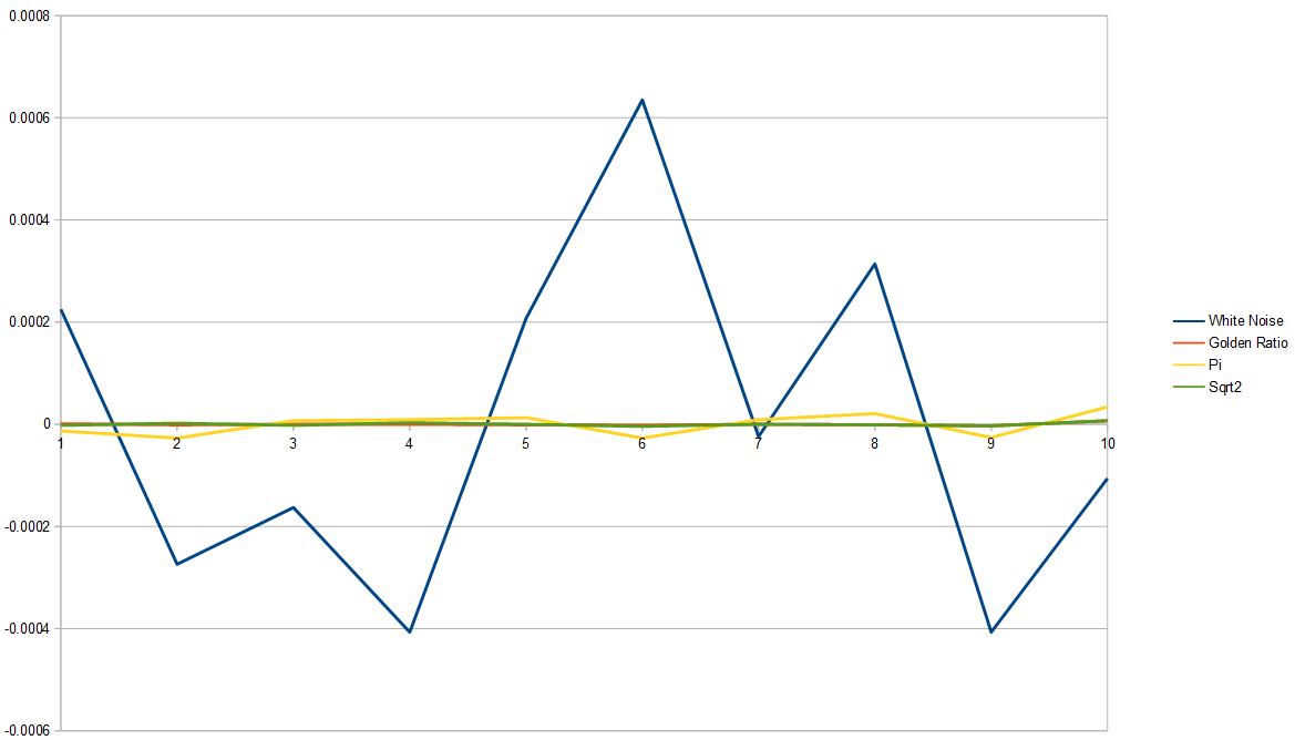
Removing white noise from that graph, we can see that pi is worst, golden ratio is best, and square root of 2 isn’t far behind the golden ratio.

Old Closing (Before Alias Table Section Added)

If you look at the code, you might be saying to yourself that the weighted version isn’t great because you need a loop to convert the 1D floating point value in [0,1] to the weighted item chosen. If you switched to using an alias table, it’d be an O(1) constant time operation, but then the 1D value would not be enough – you’d need a 1d value and a biased coin flip. AKA just a 2d value that is [0,1] on each axis. It would be interesting to compare an alias table / 2D LDS sequence to see how it converged versus this method. I really, really, should have done that in this post and should do it soon.

Another option though would be to use a “branchless, fixed step count, binary search” which would also be a constant time lookup. Basically, if you had 16 items you were searching through, you can do it with four branchless operations. This is great for shaders, SIMD programming, hardware, and similar. You can read more about that technique in my post here: https://blog.demofox.org/2017/06/20/simd-gpu-friendly-branchless-binary-search/

Alias Tables & 2D Low Discrepancy Sequences

This section shows the effect of using 2d low discrepancy sequences with an alias table to find the weighted item in constant time O(1), instead of having to loop through the weights to find the correct item.

Using an alias table is faster, but having to use 2d low discrepancy sequences instead of 1d has the possibility to change things. The concept of evenly spaced and similar ideas gets a lot more open to interpretation when you leave the first dimension.

So, first things first, here’s a graph of 1d white noise compared with 2d white noise used to do a lookup into an alias table, for 10,000 samples. This is to show that the alias table works just like not using one, and that we are doing apples to apples comparisons. I’ve also added a “weights” to the graphs as the actual ground truth of the histogram, instead of relying on sequential which was imperfect.

I’m using three 2d low discrepancy sequences. They are:

1. R2 – a generalization of the golden ratio to 2 dimensions. (more info here: http://extremelearning.com.au/unreasonable-effectiveness-of-quasirandom-sequences/)
2. Sobol – a very strong and well known LDS, which is often the best LDS shown in the papers i’ve seen (except when reading blue noise papers, but that’s a different usage case and quality metric hehe)
3. Golden Ratio / Square root of 2 – I use the golden ratio sequence on the x axis and the square root of 2 sequence on the y axis.

Here are the histograms for 100 samples, comparing the 3 LDSs vs white noise and the actual weights. 1D golden ratio is also here to compare how the 2d alias method techniques compare to the 1d golden ratio sampling. It seems to be showing that white noise and Sobol are the worst outliers, and everything else is better behaved.

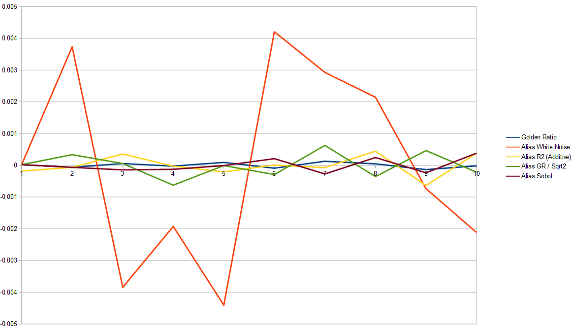
Here are 10,000 samples. I’m switching to error (subtracted out “weights”) so it’s easier to see small differences. Now alias table white noise is the single outlier, and everything else seems to be playing pretty nicely and all just about even.

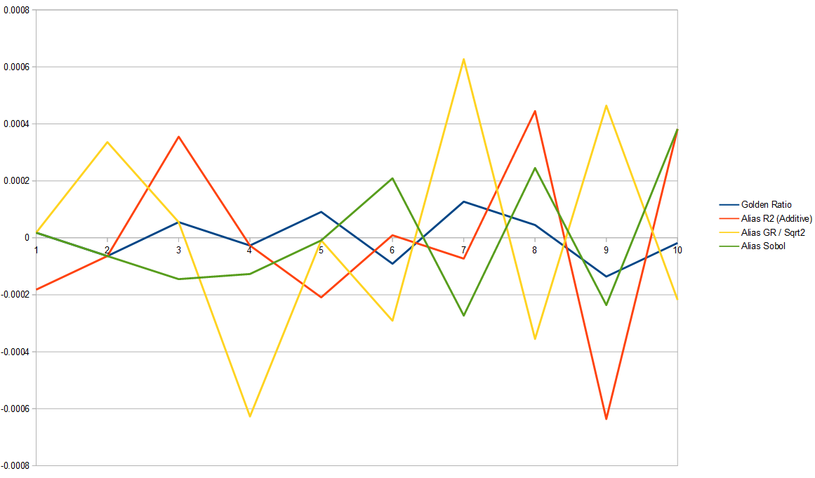
If we remove white noise we can zoom in and see things a little better. It looks like 1D golden ratio is the best, then Sobol. It’s hard to tell, but R2 seems like it might be doing better than golden ratio / square root of 2.

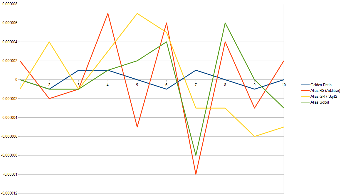
Here is the same for one million samples. 1D golden ratio seems to be the winner here and the others all seem to be doing about as well as each other.

Conclusion: If you are using an alias table, you definitely should use a decent 2d low discrepancy sequence. However, it looks like you will not do as well quality wise, as using 1d golden ratio sampling without an alias table. Maybe there is a different sampling pattern to use in the alias table case that will do better though. If you know of such a thing, please share!

I wanted to show one more thing though before we go. You might notice the graphs all call R2 “additive”. If you are wondering why that is, it’s this 2D irrational low discrepancy sequence can be calculated two different ways, just like the 1D golden ratio low discrepancy sequence can. You can either multiply an index by the irrational number(s) and fract it to get the result, or you can start at index 1, add the irrational number(s) in, fract it, then go to index 2, repeating until you get to the index you want.

Doing it the first way with a multiply causes you to run into numerical issues (error due to floating point rounding, due to finite memory storage for floats), while the second has better precision. The second way is “additive” and i want to show you just how big a difference this makes by showing you the error of both kinds after 1 million samples, along with the error for white noise.

The error from r2 done via multiplication is so large that it dwarves even the error from white noise. It isn’t as noticeable at lower sample counts, because the floating point numbers are smaller, so will hit less severe rounding problems, but it still exists at lower sample counts. This isn’t unique to R2 either… this is true of any irrational additive recurrence low discrepancy sequence (including the 1D golden ratio sequence).

You probably would have better luck with doubles.

Another thing you can do is make it into a fixed point “unsigned int” representation of the irrational so that you don’t waste storage bits on features you don’t need from floats. More info on that here:
http://marc-b-reynolds.github.io/distribution/2020/01/24/Rank1Pre.html

Links

If you found this post interesting, you might like this other post, which talks about using LDS and blue noise for making loot drop tables, and how that helps the average player experience be more predictable, compared to regular old random numbers.

“Using Low Discrepancy Sequences & Blue Noise in Loot Drop Tables for Games”
https://blog.demofox.org/2020/03/01/using-low-discrepancy-sequences-blue-noise-in-loot-drop-tables-for-games/

There is a great video from numberphile that talks about why the golden ratio is the most irrational number. Check it out 🙂

When making the alias table, i used the stable Vose method from this page: https://www.keithschwarz.com/darts-dice-coins/

Posts in this series:

1. Basic Camera, Diffuse, Emissive
2. Image Improvement and Glossy Reflections
3. Fresnel, Rough Refraction & Absorption, Orbit Camera

Below is a screenshot of the shadertoy that goes with this post. Click to view full size. That shadertoy can be found at:
https://www.shadertoy.com/view/ttfyzN

On the menu today is:

• Fresnel – This makes objects shinier at grazing angles which increases realism.
• Rough Refraction & Absorption – This makes it so we can have transparent objects, for various definitions of the term transparent.
• Orbit Camera – This lets you control the camera with the mouse to be able to see the scene from different angles

Fresnel

First up is the fresnel effect. I said I wasn’t going to do it in this series, but it really adds a lot to the end result, and we are going to need it (and related parameters) for glossy reflections anyways.

Fresnel makes objects shinier when you view them at grazing angles and helps objects look more realistic. In the image below, the left sphere does not have fresnel, but the right sphere does. Fresnel adds a better sense of depth and shape.

The fresnel function we are going to use is this, so put this in common or buffer A above the raytracing shading code.

float FresnelReflectAmount(float n1, float n2, vec3 normal, vec3 incident, float f0, float f90)
{
        // Schlick aproximation
        float r0 = (n1-n2) / (n1+n2);
        r0 *= r0;
        float cosX = -dot(normal, incident);
        if (n1 > n2)
        {
            float n = n1/n2;
            float sinT2 = n*n*(1.0-cosX*cosX);
            // Total internal reflection
            if (sinT2 > 1.0)
                return f90;
            cosX = sqrt(1.0-sinT2);
        }
        float x = 1.0-cosX;
        float ret = r0+(1.0-r0)*x*x*x*x*x;

        // adjust reflect multiplier for object reflectivity
        return mix(f0, f90, ret);
}

n1 is the “index of refraction” or “IOR” of the material the ray started in (air, and we are going to use 1.0). n2 is the “index of refraction” of the material of the object being hit. normal is the normal of the surface where the ray hit. incident is the ray direction when it hit the object. f0 is the minimum reflection of the object (when the ray and normal are 0 degrees apart), f90 is the maximum reflection of the object (when the ray and normal are 90 degrees apart).

For the index of refraction of objects, i used a value of “1.0” in the image with the 2 orange spheres above. for f90, the maximum reflection of the objects, we are going to just use “1.0” to make objects fully reflective at the edge.

Below are spheres with a minimum reflection (reflection chance!) of 0.02, and the IOR go from 1 (on the left) to 2 (on the right). To me, the one on the right looks like a pearl. (this is the SCENE define value 2 scene in the shadertoy)

To apply fresnel to our shader, find this code:

// calculate whether we are going to do a diffuse or specular reflection ray 
float doSpecular = (RandomFloat01(rngState) < hitInfo.material.percentSpecular) ? 1.0f : 0.0f;

Change it to this:

// apply fresnel
float specularChance = hitInfo.material.percentSpecular;
if (specularChance > 0.0f)
{
    specularChance = FresnelReflectAmount(
        1.0,
        hitInfo.material.IOR,
        rayDir, hitInfo.normal, hitInfo.material.percentSpecular, 1.0f);  
}
      
// calculate whether we are going to do a diffuse or specular reflection ray 
float doSpecular = (RandomFloat01(rngState) < specularChance) ? 1.0f : 0.0f;

Besides that, a float for "IOR" needs to be added to SMaterialInfo too. Here is the scene from the end of last chapter, using fresnel and with everything using an IOR of 1.0.

And here is the scene from last chapter without fresnel. The difference is pretty subtle so you might want to open each image in a browser tab to flip back and forth. The biggest difference is on the edges of the yellow and pink sphere. Fresnel makes the biggest difference for objects that are a little bit shiny. Objects that are very shiny or not at all shiny won't have as noticeable fresnel effects.

Better Diffuse / Specular Selection

In the last post we used a random number tested against a percent chance for specular to choose whether a reflected ray was going to be a diffuse ray or a specular ray.

When doing that, we should have also divided the throughput by the probability of the ray actually chosen (to not make one count more than the other in the final average) but we didn’t do that. This is a “mathy detail” but easy enough to put in casually, so let’s do the right thing.

Find the place where the doSpecular float is set based on the random roll. Put this underneath that:

// get the probability for choosing the ray type we chose
float rayProbability = (doSpecular == 1.0f) ? specularChance : 1.0f - specularChance;
        
// avoid numerical issues causing a divide by zero, or nearly so (more important later, when we add refraction)
rayProbability = max(rayProbability, 0.001f);     

Then put this right before doing the russian roulette:

// since we chose randomly between diffuse and specular,
// we need to account for the times we didn't do one or the other.
throughput /= rayProbability;

The biggest difference from the previous image is that the pink and yellow spheres brighten up a bit, and so do their reflections, of course!

Rough Refraction & Absorption

Time for the fun! We’ll talk about the features and show the results in this section, then show how to get them into the path tracer in the next section.

Thinking about the last post for a second… in simple rendering, and old style raytracers, reflection works by using the reflect() formula/function to find the perfectly sharp mirror reflection angle for a ray hitting a surface, and traces that ray. In the last post we showed how to inject some randomness into that reflected ray, by using a material roughness value to lerp between the perfectly reflected ray and a random ray over the normal oriented hemisphere.

For refraction we are going to do much the same thing.

For simple rendering and old style raytracers, there is a refract() formula/function that find a perfectly sharp refraction angle for a ray hitting a surface, where that surface has a specific IOR (Index of refraction. Same parameter as used for fresnel). The only difference is that since refracted rays go THROUGH an object instead of reflecting off an object, the random hemisphere is going to be oriented with the negative normal of the surface.

Below is an image of refractive spheres going from IOR 1 on the left, to 1.5 on the right. Notice how the background gets distorted as the IOR increases, and also notice how the light under the spheres gets focused. Those are “caustics” and get way more interesting with other shaped meshes. (this is SCENE define value 1 in the shadertoy)

You might notice some dark streaks on the ground under the spheres in the middle. When i first saw these, i thought it was a bug, but through experimentation found out that they are actually projections of the images in the sky (the top of the skybox).

To further demonstrate this, here’s a scene where the spheres are all the same IOR but they are different distances from the floor, which focuses/defocuses the image projected through the sphere, as well as the light above the spheres. (SCENE define value 4 in the shadertoy)

Changing the skybox, it looks like this. Notice the projection on the ground at the left has that circle shape?

Looking up into at what is above the spheres you can see that circle that was projected onto the ground. This is one of the coolest things about path tracing… you get a lot of techniques “for free” that are just emergent features of the math. It’s a lot different than approaching graphics in rasterization / non path traced rendering, where every feature you want, you basically have to make explicit code for to approximate.

Going back to roughness, here are some refractive spheres using an IOR of 1.1, but varying in roughness from 0 on the left, to 0.5 on the right. Notice that the spheres themselves get obviously more rough, but also their shadow / caustics change with roughness too. (SCENE define value 6 in the shadertoy)

It’s important to notice that in these, it’s just the SURFACE of the sphere that has any roughness to it. If you were able to take one of these balls and crack it in half, the inside would be completely smooth and transparent. In a future post (next, i think!) we’ll talk about how to make some roughness inside of objects, which is also how you render smoke, fog, clouds, and also things like skin, milk, and wax.

Another fun feature you can add to transparent objects is “absorption” which means that light is absorbed over distance as it travels through the object.

We’re going to use Beer’s law to get a multiplier for light that travels through the object, to make that light decrease. The formula for that is just this:

For that, we can use a different absorption value per color channel so that different colors absorb quicker or slower as the light goes through the object.

Here are some spheres that have progressively more absorption. A percentage multiplier goes from 0 on the left to 1 on the right and is multiplied by (1.0, 2.0, 3.0) to get the absorption value. Notice how the spheres change but so do the caustics / shadows. This is SCENE define value 3 in the shadertoy.

You can combine roughness and absorption to make some interesting things. Here is the same spheres but with some absorption (SCENE define value 0).

Here’s the same scene from a different view, which shows how rich the shading for these objects are.

Implementing Rough Refraction & Absorption

Let’s implement this stuff!

The first thing to do is to add more fields to our SMaterialInfo struct.

We should have something roughly like this right now:

struct SMaterialInfo
{
    vec3 albedo;           // the color used for diffuse lighting
    vec3 emissive;         // how much the surface glows
    float percentSpecular; // percentage chance of doing specular instead of diffuse lighting
    float roughness;       // how rough the specular reflections are
    vec3 specularColor;    // the color tint of specular reflections
    float IOR;             // index of refraction. used by fresnel and refraction.
};

Change it to this:

struct SMaterialInfo
{
    // Note: diffuse chance is 1.0f - (specularChance+refractionChance)
    vec3  albedo;              // the color used for diffuse lighting
    vec3  emissive;            // how much the surface glows
    float specularChance;      // percentage chance of doing a specular reflection
    float specularRoughness;   // how rough the specular reflections are
    vec3  specularColor;       // the color tint of specular reflections
    float IOR;                 // index of refraction. used by fresnel and refraction.
    float refractionChance;    // percent chance of doing a refractive transmission
    float refractionRoughness; // how rough the refractive transmissions are
    vec3  refractionColor;     // absorption for beer's law    
};

You might notice that there is both a specular roughness as well as a refraction roughness. That could be combined into a single “surface roughness” which was used by both if desired. You lose the ability to make reflections have different roughness than refraction, but that wouldn’t be a huge loss.

Also, there is a specular chance, and refraction chance, with an implied diffuse chance making those sum to 1.0.

Instead of doing chances that way, another thing to try could be to make the diffuse chance be the sum of the albedo components, the specular chance be the sum of the specular color components, and the refraction chance be the sum of refraction color components. You could then divide them all by the sum of all 3 chances, so that they summed up to 1.0.

This would let you get rid of those percentages, and should be pretty good choices. The only weird thing is that the meaning of refraction color is sort of reversed compared to the others. The others are how much light to let through, but refraction color is how much light to block. You might have better luck subtracting refraction color from (1,1,1) and using that to make a refraction chance.

Since the light from rays is divided by the probability of choosing that type of ray (diffuse, specular, or refractive), it doesn’t really matter how you choose the probabilities for choosing the ray type, but when the probabilities better match the contribution to the pixel’s final color (more contribution = higher percentage), you are going to get a better (more converged) image more quickly. This is straight up importance sampling, and i’ll stop there so we can keep this casual 🙂

The next change is to address a problem we are likely to hit. Now that our material has quite a few components, it would be real easy to forget to set one when setting material properties. If you ever forget to set one, you are either going to have uninitialized values, or values coming from a previous ray hit that is no longer valid. That is going to make some real hard to track bugs, along with the possibility of undefined behavior due to uninitialized values (AFAIK). So, I made a function that initializes a material roughly to zero, but mainly just to sane values. The idea is that you call this function to init a material, and then set the specific values you care about.

SMaterialInfo GetZeroedMaterial()
{
    SMaterialInfo ret;
    ret.albedo = vec3(0.0f, 0.0f, 0.0f);
    ret.emissive = vec3(0.0f, 0.0f, 0.0f);
    ret.specularChance = 0.0f;
    ret.specularRoughness = 0.0f;
    ret.specularColor = vec3(0.0f, 0.0f, 0.0f);
    ret.IOR = 1.0f;
    ret.refractionChance = 0.0f;
    ret.refractionRoughness = 0.0f;
    ret.refractionColor = vec3(0.0f, 0.0f, 0.0f);
    return ret;
}

Every time i set material info (like, every time a ray intersection passes), i first call this function, and then set the specific values I care about. I also call it on the SRayHitInfo struct itself when i first declare it in GetColorForRay().

Next, also add a bool “fromInside” to the SRayHitInfo. We are going to need this to know when we intersect an object if we hit it from the inside, or the outside. Refraction made it so we can go inside of objects, and we need to know when that happens now.

struct SRayHitInfo
{
    bool fromInside;
    float dist;
    vec3 normal;
    SMaterialInfo material;
};

In TestQuadTrace(), where it modifies the ray hit info, make sure and set fromInside to false. We are going to say there is no inside to a quad. You could make it so the negative side of the quad (based on it’s normal) was inside, and maybe build boxes etc out of quads, but I decided not to deal with that complexity.

TestSphereTrace() already has the concept of whether the ray hit the sphere from the inside or not, but it doesn’t expose it to the caller. I just have it set the ray hit info fromInside bool based on that fromInside bool that already exists.

The various uses of roughness and percentSpecular are going to need to change to specularRoughness and specularChance.

The final shading inside the bounce for loop changes quite a bit so i’m going to just paste this below, but it is commented pretty heavily so hopefully makes sense.

The biggest thing worth explaining I think is how absorption happens. We don’t know how much absorption is going to happen when we enter an object because we don’t know how far the ray will travel through the object. Because of this, we can’t change the throughput to account for absorption when entering an object. We need to instead wait until we hit the far side of the object and then can calculate absorption and update the throughput to account for it. Another way of looking at this is that “when we hit an object from the inside, it means we should calculate and apply absorption”. This also handles the case of where a ray might bounce around inside of an object multiple times before leaving (due to specular reflection and fresnel happening INSIDE an object) – absorption would be calculated and applied at each internal specular bounce.

for (int bounceIndex = 0; bounceIndex < = c_numBounces; ++bounceIndex)
{
    // shoot a ray out into the world
    SRayHitInfo hitInfo;
    hitInfo.material = GetZeroedMaterial();
    hitInfo.dist = c_superFar;
    hitInfo.fromInside = false;
    TestSceneTrace(rayPos, rayDir, hitInfo);
    
    // if the ray missed, we are done
    if (hitInfo.dist == c_superFar)
    {
        ret += SRGBToLinear(texture(iChannel1, rayDir).rgb) * c_skyboxBrightnessMultiplier * throughput;
        break;
    }
    
    // do absorption if we are hitting from inside the object
    if (hitInfo.fromInside)
        throughput *= exp(-hitInfo.material.refractionColor * hitInfo.dist);
    
    // get the pre-fresnel chances
    float specularChance = hitInfo.material.specularChance;
    float refractionChance = hitInfo.material.refractionChance;
    //float diffuseChance = max(0.0f, 1.0f - (refractionChance + specularChance));
    
    // take fresnel into account for specularChance and adjust other chances.
    // specular takes priority.
    // chanceMultiplier makes sure we keep diffuse / refraction ratio the same.
    float rayProbability = 1.0f;
    if (specularChance > 0.0f)
    {
        specularChance = FresnelReflectAmount(
            hitInfo.fromInside ? hitInfo.material.IOR : 1.0,
            !hitInfo.fromInside ? hitInfo.material.IOR : 1.0,
            rayDir, hitInfo.normal, hitInfo.material.specularChance, 1.0f);
        
        float chanceMultiplier = (1.0f - specularChance) / (1.0f - hitInfo.material.specularChance);
        refractionChance *= chanceMultiplier;
        //diffuseChance *= chanceMultiplier;
    }
    
    // calculate whether we are going to do a diffuse, specular, or refractive ray
    float doSpecular = 0.0f;
    float doRefraction = 0.0f;
    float raySelectRoll = RandomFloat01(rngState);
    if (specularChance > 0.0f && raySelectRoll < specularChance)
    {
        doSpecular = 1.0f;
        rayProbability = specularChance;
    }
    else if (refractionChance > 0.0f && raySelectRoll < specularChance + refractionChance)
    {
        doRefraction = 1.0f;
        rayProbability = refractionChance;
    }
    else
    {
        rayProbability = 1.0f - (specularChance + refractionChance);
    }
    
    // numerical problems can cause rayProbability to become small enough to cause a divide by zero.
    rayProbability = max(rayProbability, 0.001f);
    
    // update the ray position
    if (doRefraction == 1.0f)
    {
        rayPos = (rayPos + rayDir * hitInfo.dist) - hitInfo.normal * c_rayPosNormalNudge;
    }
    else
    {
        rayPos = (rayPos + rayDir * hitInfo.dist) + hitInfo.normal * c_rayPosNormalNudge;
    }
     
    // Calculate a new ray direction.
    // Diffuse uses a normal oriented cosine weighted hemisphere sample.
    // Perfectly smooth specular uses the reflection ray.
    // Rough (glossy) specular lerps from the smooth specular to the rough diffuse by the material roughness squared
    // Squaring the roughness is just a convention to make roughness feel more linear perceptually.
    vec3 diffuseRayDir = normalize(hitInfo.normal + RandomUnitVector(rngState));
    
    vec3 specularRayDir = reflect(rayDir, hitInfo.normal);
    specularRayDir = normalize(mix(specularRayDir, diffuseRayDir, hitInfo.material.specularRoughness*hitInfo.material.specularRoughness));

    vec3 refractionRayDir = refract(rayDir, hitInfo.normal, hitInfo.fromInside ? hitInfo.material.IOR : 1.0f / hitInfo.material.IOR);
    refractionRayDir = normalize(mix(refractionRayDir, normalize(-hitInfo.normal + RandomUnitVector(rngState)), hitInfo.material.refractionRoughness*hitInfo.material.refractionRoughness));
            
    rayDir = mix(diffuseRayDir, specularRayDir, doSpecular);
    rayDir = mix(rayDir, refractionRayDir, doRefraction);
    
    // add in emissive lighting
    ret += hitInfo.material.emissive * throughput;
    
    // update the colorMultiplier. refraction doesn't alter the color until we hit the next thing, so we can do light absorption over distance.
    if (doRefraction == 0.0f)
        throughput *= mix(hitInfo.material.albedo, hitInfo.material.specularColor, doSpecular);
    
    // since we chose randomly between diffuse, specular, refract,
    // we need to account for the times we didn't do one or the other.
    throughput /= rayProbability;
    
    // Russian Roulette
    // As the throughput gets smaller, the ray is more likely to get terminated early.
    // Survivors have their value boosted to make up for fewer samples being in the average.
    {
        float p = max(throughput.r, max(throughput.g, throughput.b));
        if (RandomFloat01(rngState) > p)
            break;

        // Add the energy we 'lose' by randomly terminating paths
        throughput *= 1.0f / p;            
    }
}

Orbit Camera

Now that we can do all these cool renders, it kind of sucks that the camera is stuck in one place.

It really is a lot of fun being able to move the camera around and look at things from different angles. It’s also really helpful in debugging – like when we were able to see the circle on the ceiling of the skybox!

Luckily an orbit camera is pretty easy to add!

First drop this function in the buffer A tab, right above the mainImage function. You can leave the constants there or put them into the common tab, whichever you’d rather do.

// mouse camera control parameters
const float c_minCameraAngle = 0.01f;
const float c_maxCameraAngle = (c_pi - 0.01f);
const vec3 c_cameraAt = vec3(0.0f, 0.0f, 20.0f);
const float c_cameraDistance = 20.0f;

void GetCameraVectors(out vec3 cameraPos, out vec3 cameraFwd, out vec3 cameraUp, out vec3 cameraRight)
{
    // if the mouse is at (0,0) it hasn't been moved yet, so use a default camera setup
    vec2 mouse = iMouse.xy;
    if (dot(mouse, vec2(1.0f, 1.0f)) == 0.0f)
    {
        cameraPos = vec3(0.0f, 0.0f, -c_cameraDistance);
        cameraFwd = vec3(0.0f, 0.0f, 1.0f);
        cameraUp = vec3(0.0f, 1.0f, 0.0f);
        cameraRight = vec3(1.0f, 0.0f, 0.0f);
        return;
    }
    
    // otherwise use the mouse position to calculate camera position and orientation
    
    float angleX = -mouse.x * 16.0f / float(iResolution.x);
    float angleY = mix(c_minCameraAngle, c_maxCameraAngle, mouse.y / float(iResolution.y));
    
    cameraPos.x = sin(angleX) * sin(angleY) * c_cameraDistance;
    cameraPos.y = -cos(angleY) * c_cameraDistance;
    cameraPos.z = cos(angleX) * sin(angleY) * c_cameraDistance;
    
    cameraPos += c_cameraAt;
    
    cameraFwd = normalize(c_cameraAt - cameraPos);
    cameraRight = normalize(cross(vec3(0.0f, 1.0f, 0.0f), cameraFwd));
    cameraUp = normalize(cross(cameraFwd, cameraRight));   
}

The mainImage function also changes quite a bit between the seeding of rng and the raytracing – basically the stuff that controls jitter for TAA and calculates the camera vectors. The whole function is below, hopefully well enough commented to understand.

void mainImage( out vec4 fragColor, in vec2 fragCoord )
{
    // initialize a random number state based on frag coord and frame
    uint rngState = uint(uint(fragCoord.x) * uint(1973) + uint(fragCoord.y) * uint(9277) + uint(iFrame) * uint(26699)) | uint(1);    
    
    // calculate subpixel camera jitter for anti aliasing
    vec2 jitter = vec2(RandomFloat01(rngState), RandomFloat01(rngState)) - 0.5f;

    // get the camera vectors
    vec3 cameraPos, cameraFwd, cameraUp, cameraRight;
    GetCameraVectors(cameraPos, cameraFwd, cameraUp, cameraRight);    
    vec3 rayDir;
    {   
        // calculate a screen position from -1 to +1 on each axis
        vec2 uvJittered = (fragCoord+jitter)/iResolution.xy;
        vec2 screen = uvJittered * 2.0f - 1.0f;
        
        // adjust for aspect ratio
        float aspectRatio = iResolution.x / iResolution.y;
        screen.y /= aspectRatio;
                
        // make a ray direction based on camera orientation and field of view angle
        float cameraDistance = tan(c_FOVDegrees * 0.5f * c_pi / 180.0f);       
        rayDir = vec3(screen, cameraDistance);
        rayDir = normalize(mat3(cameraRight, cameraUp, cameraFwd) * rayDir);
    }
    
    // raytrace for this pixel
    vec3 color = vec3(0.0f, 0.0f, 0.0f);
    for (int index = 0; index  0.1);
    
    // average the frames together
    vec4 lastFrameColor = texture(iChannel0, fragCoord / iResolution.xy);
    float blend = (iFrame  0.0 || lastFrameColor.a == 0.0f || spacePressed) ? 1.0f : 1.0f / (1.0f + (1.0f / lastFrameColor.a));
    color = mix(lastFrameColor.rgb, color, blend);

    // show the result
    fragColor = vec4(color, blend);
}

After you’ve done that, you can drag the left mouse in the image to move the camera around 🙂

If you follow these steps with the scene from last post, and change the central sphere to be a bit refractive, you can finally view the box from a different angle!

Closing

Before we go, I want to show some refractive spheres with IOR 1, refraction roughness 0, but fading between a purely refractive surface on the left, to a purely diffuse surface on the right. This is SCENE define value 5 in the shadertoy.

Compare this one to the purely absorption scene shown before, and also the purely roughness scene.

All of these 3 obscured what was behind them more as the effect was turned up. All of them also could have the effect partially in effect, to any level.

So, all 3 of these examples were semi transparent.

Which of these is it we are talking about when we are doing traditional alpha blending in a rasterized scene?

Well it turns out to be a bit ambiguous.

If the shadow of a semi transparent object is colored, that means absorption is the best model for it. If the shadow of a semi transparent object is just darkened, the partially diffuse surface may be the best model (could also be absorption though). If the object doesn’t cast a shadow (or barely does), it is an object made semi transparent by roughness on the surface of the object, or INSIDE the object (we’ll talk about that case later). That is especially true if the appearance (lighting) of the object changes significantly when the lighting behind it (or around it) changes, vs an object which is only lit from the front.

Kind of a strange thing thinking about alpha as all these different effects, but good to be aware of it too if doing realistic rendering.

Who knew transparency would be so opaque?

Oh PS – a color tip I got from an artist once was to never use pure primary colors (I think it was Ron Harvey @ monolith. If you are reading this Ron, hello!). This is nice from an artistic standpoint, but also, if you think about how lighting is multiplied by these various colors, whenever you make any color channel 0, it means none of that color channel will make it through that multiplication. Completely killing light of any kind feels wrong and does make things look subtly wrong (or not subtly!), because nothing in the real world is so perfect or pure that it doesn’t reflect SOME light of a different frequency than it’s main frequency or frequencies. If it were so impossibly pure, dust would fall on it and change that. Also, it’s probably a good idea to stay away from 1 for similar reasons – nothing perfectly reflects anything in the real world, there is always some imperfection – again, if it were, dust would fall on it and change it.

I think volumetrics and depth of field are next 🙂

Thanks for reading, and i’d love to see anything you make. You can find me at @Atrix256

Posts in this series:

1. Basic Camera, Diffuse, Emissive
2. Image Improvement and Glossy Reflections
3. Fresnel, Rough Refraction & Absorption, Orbit Camera

Below is a screenshot of the shadertoy that goes with this post. Click to view full size. That shadertoy can be found at:
https://www.shadertoy.com/view/WsBBR3

In this blog post we are going to improve the quality of our rendered image from last time, and also add specular / glossy reflections, to end up with the image above. Compare that to the image below, which is where we are starting from, after part 1.

On the menu today is…

• Anti Aliasing – This makes pixelated edges be smooth, which makes for a much better render
• sRGB – The space we do lighting calculations in are not the same as the display wants. This fixes that.
• Tone Mapping – This converts unbounded lighting to a displayable range.
• Exposure – This lets us brighten or darken our image before tone mapping, just like a camera’s exposure setting does.
• Glossy Reflections – We make some objects shiny

Anti Aliasing

Adding anti aliasing to a path tracer is super easy. All we need to do is add a random number between -0.5 and +0.5 to our pixel’s location, on the x and y axis.

Since the pixel color is the average over lots of frames, what this does is give us the “average color of the pixel”. That means if the edge of a shape goes through a pixel, the pixel will average the color of the shape, and also the color of whatever is in the background. That gives us smooth anti aliased edges.

To do this, find this code:

// calculate coordinates of the ray target on the imaginary pixel plane.
// -1 to +1 on x,y axis. 1 unit away on the z axis
vec3 rayTarget = vec3((fragCoord/iResolution.xy) * 2.0f - 1.0f, cameraDistance);

and replace it with this:

// calculate subpixel camera jitter for anti aliasing
vec2 jitter = vec2(RandomFloat01(rngState), RandomFloat01(rngState)) - 0.5f;
    
// calculate coordinates of the ray target on the imaginary pixel plane.
// -1 to +1 on x,y axis. 1 unit away on the z axis
vec3 rayTarget = vec3(((fragCoord+jitter)/iResolution.xy) * 2.0f - 1.0f, cameraDistance);

Doing that gives us this image below. You might want to click to view it full size and compare it vs last image, to see how the edges of the spheres are smooth now. Viewing the smaller image hides the pixelation.

sRGB

The colors that we send to a display are not the same as the colors that we see. This is because human vision is not linear.

With only 256 shades of color in 8 bit per color channel images, if we split the shades evenly, we’d find that there wasn’t enough dark shades because our eyes can see more detail in darker shades.

To make up for this, sRGB was made, which makes it so the values between 0 and 255 are not linearly spaced – there are more values in darker colors and less in the lighter colors.

If we do our lighting calculations in sRGB though, the math doesn’t work right because there was a non linear transform applied to our color channels.

To fix this, whenever we read a color from a texture, we should convert from sRGB to linear. Also, whenever we write out a pixel, we want to convert from linear to sRGB so it shows up correctly on the display.

We need to add these functions to our shadertoy. Make a new “common” tab and put it in there. The common tab is a header included by all other tabs, so things we put there are usable by all other tabs. In the shader that goes with this post, i put many utility functions, constants, and user controllable parameters in the common tab.

vec3 LessThan(vec3 f, float value)
{
    return vec3(
        (f.x < value) ? 1.0f : 0.0f,
        (f.y < value) ? 1.0f : 0.0f,
        (f.z < value) ? 1.0f : 0.0f);
}

vec3 LinearToSRGB(vec3 rgb)
{
    rgb = clamp(rgb, 0.0f, 1.0f);
    
    return mix(
        pow(rgb, vec3(1.0f / 2.4f)) * 1.055f - 0.055f,
        rgb * 12.92f,
        LessThan(rgb, 0.0031308f)
    );
}

vec3 SRGBToLinear(vec3 rgb)
{
    rgb = clamp(rgb, 0.0f, 1.0f);
    
    return mix(
        pow(((rgb + 0.055f) / 1.055f), vec3(2.4f)),
        rgb / 12.92f,
        LessThan(rgb, 0.04045f)
	);
}

ERRATA SRGBToLinear() just returned the input, in the original version of this post. That was incorrect, and correcting that changes the results you get from here on out. The only thing using the function was the skybox lookup, but that means you will get different results than are shown in the screenshots here. The problem isn’t on your end, it’s mine. Sorry about that! In fact, instead of skybox lighting being too bright as i talk about later on and having to multiply it by 0.5, it ends up being too dim and in the final shader you’ll see i multiply it by 2. Apologies and thank you for reading 🙂

There are two places we need to use this functionality. The first place is where we read the cube map when rays miss the scene geometry.

Find this code:

// if the ray missed, we are done
if (hitInfo.dist == c_superFar)
{
    ret += texture(iChannel1, rayDir).rgb * throughput;
    break;
}

Change it to this:

// if the ray missed, we are done
if (hitInfo.dist == c_superFar)
{
    ret += SRGBToLinear(texture(iChannel1, rayDir).rgb) * throughput;
    break;
}

The other place we want to change is where we write the final pixel color out.

In the “Image” tab, find this code:

vec3 color = texture(iChannel0, fragCoord / iResolution.xy).rgb;

and replace it with this:

vec3 color = texture(iChannel0, fragCoord / iResolution.xy).rgb;

// convert from linear to sRGB for display
color = LinearToSRGB(color);

Doing that, we get this image:

You might notice the balls changed color significantly. That’s because they were sRGB colors before but now they are linear colors. We can adjust their colors to make them look better though. If we change the 0.75s if their albedo to 0.5s, that gives us an image like this:

Tone Mapping & Exposure

The next thing to tackle is the fact that when we are calculating lighting, the range of light goes from 0 (perfect black) up to an unbounded amount of brightness, but our display can only display values between 0 and 1.

Tone mapping is the process of remapping the values to the 0 to 1 range. Tone mapping preserves detail in the darks while also making pixels that are too bright also have recognizable detail. We are going to use a luminance only fit of the ACES tone mapper. This tone mapping code was made by Krzysztof Narkowicz and you can read more about it on his website: https://knarkowicz.wordpress.com/2016/01/06/aces-filmic-tone-mapping-curve/

Here is the function to put in the common tab:

// ACES tone mapping curve fit to go from HDR to LDR
//https://knarkowicz.wordpress.com/2016/01/06/aces-filmic-tone-mapping-curve/
vec3 ACESFilm(vec3 x)
{
    float a = 2.51f;
    float b = 0.03f;
    float c = 2.43f;
    float d = 0.59f;
    float e = 0.14f;
    return clamp((x*(a*x + b)) / (x*(c*x + d) + e), 0.0f, 1.0f);
}

That function takes linear color in and gives linear color out, so we need to call it after we get the raw color, but before we convert that color to sRGB, in the image tab.

    vec3 color = texture(iChannel0, fragCoord / iResolution.xy).rgb;

    // convert unbounded HDR color range to SDR color range
    color = ACESFilm(color);

    // convert from linear to sRGB for display
    color = LinearToSRGB(color);
    
    fragColor = vec4(color, 1.0f);

Doing that we get this image.

The lighting on the back wall has mellowed out a bit and looks a lot more natural which is nice. It still seems a bit bright though.

To fix this we are going to do 2 things. Firstly, we are going to multiply the value we read from the skybox by 0.5 to darken the sky box a little. (i won’t paste code for that, just multiply the texture value by 0.5 after converting it to linear)

Secondly, we are going to apply EXPOSURE to the scene, by multiplying the color by a value of 0.5 before we put it through the tone mapper. That makes it so the entirety of the code in the “Image” tab is this:

void mainImage( out vec4 fragColor, in vec2 fragCoord )
{
    vec3 color = texture(iChannel0, fragCoord / iResolution.xy).rgb;

    // apply exposure (how long the shutter is open)
    color *= c_exposure;

    // convert unbounded HDR color range to SDR color range
    color = ACESFilm(color);

    // convert from linear to sRGB for display
    color = LinearToSRGB(color);
    
    fragColor = vec4(color, 1.0f);
}

With those two changes, our render now looks like this:

Glossy Reflections

Now for the part that everyone is waiting for: glossy reflections to make shiny things!

If you’ve done simple lighting in shaders before, you’ve probably used reflect() to calculate a light reflection ray to do some specular highlights (shiny spots) on objects.

We are going to put albedo and emissive into a SMaterialInfo struct inside of SRayHitInfo, and we are also going to add these fields:

• percentSpecular – A float between 0 and 1. What percentage of the light that hits this object is going to be reflected specularly instead of diffusely. This is the percentage chance that a ray hitting this surface is going to choose a specular reflection instead of a diffuse one
• roughness – A float between 0 and 1. How rough the surface is, which controls how blurry the reflection is. A value of 0 is a very sharp clean mirror like reflection, and a value of 1 is so blurry it looks just like diffuse.
• specularColor – A vec3 which is the color of specular reflections, just like how albedo is the color of diffuse reflections. This lets you have different colors for diffuse and specular reflections, letting you have colored metal and similar.

Here is how our shading is going to work:

• We are going to roll a random number from 0 to 1. If it’s less than percentSpecular, we are doing a specular ray, else we are doing a diffuse ray.
• Diffuse rays use cosine weighted random hemisphere samples like before.
• A fully rough specular ray is going to use that diffuse ray direction.
• A zero roughness specular ray is going to use a ray direction calculated from reflect().
• A specular ray with roughness between 0 and 1 is going to square the roughness (personal preference, you don’t have to square it), and use that value to linearly interpolate between the specular and diffuse ray directions, normalizing the result.
• Instead of always multiplying throughput by albedo, if it’s a specular ray, we are going to instead multiply it by specularColor

That is all there is to it! Find this code:

// update the ray position
rayPos = (rayPos + rayDir * hitInfo.dist) + hitInfo.normal * c_rayPosNormalNudge;

// calculate new ray direction, in a cosine weighted hemisphere oriented at normal
rayDir = normalize(hitInfo.normal + RandomUnitVector(rngState));

// add in emissive lighting
ret += hitInfo.emissive * throughput;

// update the colorMultiplier
throughput *= hitInfo.albedo;

And replace it with this:

// update the ray position
rayPos = (rayPos + rayDir * hitInfo.dist) + hitInfo.normal * c_rayPosNormalNudge;

// calculate whether we are going to do a diffuse or specular reflection ray 
float doSpecular = (RandomFloat01(rngState) < hitInfo.material.percentSpecular) ? 1.0f : 0.0f;

// Calculate a new ray direction.
// Diffuse uses a normal oriented cosine weighted hemisphere sample.
// Perfectly smooth specular uses the reflection ray.
// Rough (glossy) specular lerps from the smooth specular to the rough diffuse by the material roughness squared
// Squaring the roughness is just a convention to make roughness feel more linear perceptually.
vec3 diffuseRayDir = normalize(hitInfo.normal + RandomUnitVector(rngState));
vec3 specularRayDir = reflect(rayDir, hitInfo.normal);
specularRayDir = normalize(mix(specularRayDir, diffuseRayDir, hitInfo.material.roughness * hitInfo.material.roughness));
rayDir = mix(diffuseRayDir, specularRayDir, doSpecular);

// add in emissive lighting
ret += hitInfo.material.emissive * throughput;

// update the colorMultiplier
throughput *= mix(hitInfo.material.albedo, hitInfo.material.specularColor, doSpecular);

If we update our scene geometry and materials a bit, we now can get the final image:

The green balls in the back have a percentSpecular of 1.0, so they are all specular. Their roughness from left to right is: 0, 0.25, 0.5, 0.75, 1.0. Their specular color is (0.3, 1.0, 0.3) which makes them have a green tint. In PBR speak, this would be a green metal (we aren't using PBR specular calculations though!).

The yellow ball in the front left has a percent specular of 0.1, a roughness of 0.2 and a specular color of (0.9f, 0.9f, 0.9f). In PBR speak, this is a dielectric.

The pinkish ball in the front center has the same except a percent specular of 0.3, so is shinnier. (Still a dielectric)

The blue and magenta ball in the front right is there to show that if you pick bad material values, you can get something that doesn't look very good. That ball has an albedo of pure blue, a percent specular of 0.5, a roughness of 0.5 and a specular color of pure red. That isn't a very realistic thing you could see in the real world – a blue object with red reflections – so it doesn't look very good in the render. Garbage in, garbage out. In PBR speak, you could get this by having a dual layer material… a blue very rough or diffuse dielectric, with a clear coat that acts like a metal? It doesn't make much sense in PBR which further shows that it isn't a very well motivated material, which is why it doesn't look very good.

If you feel like taking things a little further, our render could look better with fresnel, making glancing ray angles be more reflective. I'm not planning on doing that in this series but I do have a blog post on it here: https://blog.demofox.org/2017/01/09/raytracing-reflection-refraction-fresnel-total-internal-reflection-and-beers-law/

Bonus 1: Russian Roulette

Each ray will bounce up to 8 times, but there are times when it really doesn’t need 8 bounces to give the right look.

If we were somehow able to detect this, we could end a ray early, especially if we knew how to handle the probabilities correctly to not add bias from ending early.

Russian roulette is a method for doing just that.

We are going to find the maximum color channel value in our throughput, R, G or B, and that value will be the percentage chance that we keep going with our ray after each bounce. When we do keep going, we are going to divide our throughput by that chance of keeping the ray, which makes up for the fact that we kill some of the rays there some of the other times, by making future bounces brighter.

What this means is that as the throughput gets lower, meaning future ray bounces are likely to impact the final image less, we become more likely to stop the ray bouncing around early.

This is mainly just a performance optimization, but is good because it lets you converge faster due to being able to get more samples more quickly.

Just put this code right under where we update the throughput by multiplying it by diffuse or specular.

// Russian Roulette
// As the throughput gets smaller, the ray is more likely to get terminated early.
// Survivors have their value boosted to make up for fewer samples being in the average.
{
    float p = max(throughput.r, max(throughput.g, throughput.b));
    if (RandomFloat01(rngState) > p)
        break;

    // Add the energy we 'lose' by randomly terminating paths
    throughput *= 1.0f / p;
}

To give an idea of how this affects performance, on my machine at (i forget) resolution and (i forget) renders per frame, i was getting 30 fps which is 33.3 milliseconds per frame. After I put in this Russian roulette code, it went up to 40 fps which is 25 milliseconds per frame. Same exact visual results, but 8ms less render time per frame, or a 25% improvement in speed.

Bonus 2: Space Bar to Reset

It can be hard to get a full screen screenshot in shadertoy, because you have to click the button to make it full screen (see image below) and then it already has some of the small rendering still there on the screen.

We can actually make it so when you press the space bar, that it resets the render.

How you do this is instead of using iFrame to figure out how much to blend this frame into the next, you store the blend (1/framesRendered) in the alpha channel of each pixel. You can then assign the keyboard as a texture to iChannel2 (it’s under the Misc tab) and then read that “keyboard texture” to see if the space key was pressed.

Find this code:

// average the frames together
vec3 lastFrameColor = texture(iChannel0, fragCoord / iResolution.xy).rgb;
color = mix(lastFrameColor, color, 1.0f / float(iFrame+1));

// show the result
fragColor = vec4(color, 1.0f);

And replace it with this (after assigning the keyboard as a texture in the iChannel2 slot!):

// see if space was pressed. if so we want to restart our render.
// This is useful for when we go fullscreen for a bigger image.
bool spacePressed = (texture(iChannel2, vec2(32.5/256.0,0.25)).x > 0.1);

// average the frames together
vec4 lastFrameColor = texture(iChannel0, fragCoord / iResolution.xy);
float blend = (lastFrameColor.a == 0.0f || spacePressed) ? 1.0f : 1.0f / (1.0f + (1.0f / lastFrameColor.a));
color = mix(lastFrameColor.rgb, color, blend);

// show the result
fragColor = vec4(color, blend);

Now, you can flip to full screen and press space bar to reset the render to get a better larger render.

Closing

Don’t forget… if you are trying to make a render and you are seeing 60fps, that means you probably could be converging faster and you are waiting for no good reason. Try turning c_numRendersPerFrame up until you aren’t at 60fps anymore. Anything lower than 60 means it’s working near capacity, getting it down to 10 or 5 or lower fps isn’t going to help you, so don’t worry about bringing your shadertoy tab to a crawl, it doesn’t do any good.

Be on the lookout for the next post in this series. We have some more topics to casually implement, including: depth of field and bokeh, camera movement, participating media (fog), bloom, refraction & transparencies, and more.

Thanks for reading and share any cool things you make with me on twitter at @Atrix256

This post explains how Russian Roulette can be viewed as rejection sampling a PDF to do importance sampling.

The explanation sticks to simple 1D functions and has some ~500 lines of c++ to accompany it that made the data for the explanations.

The code is at: https://github.com/Atrix256/RussianRoulette1D

Background Topics

Here are some quick definitions and links to more info.

Monte Carlo Integration – Using random samples of a function to find the area under the curve if you graphed it. Aka using random numbers to integrate a function numerically.

Importance Sampling – Using random numbers in Monte Carlo integration where the probabilities of numbers drawn aren’t the same for each number. As the graph of the probabilities looks more similar to the graph of the function being sampled, Monte Carlo integration gets closer to the right answer a lot more quickly. At the extreme, it only takes one sample to get the exact answer!

PDF – Probability density function. This is a function that describes how probable different numbers are for being generated. It integrates to 1, but might have values that go above one. The area under the curve between 2 values is the percent chance probability of a random number falling between those two values.

Uniform Distribution – Random numbers (A PDF) where all possible values are equally likely. If you made a histogram of the numbers generated from this distribution, it would be flat, if you generated an infinite number of values.

Rejection Sampling – If you know the shape of a PDF you would like to draw random numbers from, but you aren’t sure how to actually generate random numbers following that PDF, rejection sampling is one way to do that.

Russian Roulette – If you have something like an infinitely recursive (or iterative) integral, like you find with the rendering equation, Russian Roulette is a way to stop the infinite process early while still getting the correct answer. It stops early without adding bias. More generally it lets you skip doing some of the work you have to do, without adding bias.

Here are the links:

Monte Carlo Integration Explanation in 1D

Generating Random Numbers From a Specific Distribution With Rejection Sampling

Russian Roulette and Splitting (PBRT book chapter 13.7)

You’ll also see the code for this post doing a “lerp” to average sample points. If you want more info about that, check this out:

Incremental Averaging

Integrating y=x^2 from 0 to 1

Let’s look at a couple different ways to integrate a function numerically, to get a sense of things.

We’re going to integrate y=x^2 from 0 to 1 three different ways. First we’ll use regular Monte Carlo with a uniform distribution, second we’ll importance sample it using rejection sampling, and thirdly, we’ll use Russian roulette which as you’ll see is also importance sampling using rejection sampling.

Simple Monte Carlo integration works like this:

1. Take N random samples of a function between A and B
2. Sum them up and divide by N to get the average height of the function between A and B
3. Multiply by B-A to get the area under the curve

Doing that with the accompanying code, after 1000 samples the value it comes up with is 0.298374. The actual value is 1/3 or 0.33333… so it got fairly close. Check out the “// monte carlo” section in the code inside of TestFlat().

We’ll do the same steps again but this time do importance sampling with rejection sampling.

Since we know y=x^2 is 0 when x is 0 and 1 where x is 1, we can use rejection sampling to make a probability density function that is similar.

Whenever we generate a random number “x” between 0 and 1 to use in the function, we’ll say there is an “x” percent chance that we keep that number, otherwise we throw it away and generate a new random number. Another way of saying this is that there is a 1-x percent chance that we are going to throw it away and generate a new random number.

That probability of keeping numbers looks like the function y=x when you do this. y=x isn’t a proper PDF though because the area under the curve is 0.5, not 1, so you need to multiply it by 2 to make it a proper PDF. This doesn’t actually change the probabilities, this is just making a “proper PDF” that describes the probabilities. So, the PDF for these random numbers is y=2x.

We have to change how we use these random numbers too though. After we calculate our y value by plugging x into y=x*x, we need to divide it by the PDF value for x before we add them to the sum (the sum which we later divide by N to get the average). You just plug x into the PDF function y=2x to get the PDF value. We divide by the PDF because what this does is make it so numbers that come up more often weigh less into the final average. For instance, if one number came up twice as often than another in your random numbers, you should make it count for half as much to the final average, to make things equal like they are in plain vanilla Monte Carlo.

When we do this with 1000 samples, we get a value of 0.334112 (Monte Carlo was 0.298374). You might find it interesting that we had to generate 2052 potential x values for the 1000 we actually used. 1052 were thrown away.

Next up we are going to do Russian Roulette. How this works is we are going to have a probability where we just aren’t going to take a sample AT ALL. We are going to modify the first step of the Monte Carlo algorithm:

1. Take N random samples of a function between A and B. There is some percent chance “p” we won’t actually do a sample, but will just use a value of 0. If we do take a sample, we are going to divide the value we got by 1-p which will make it a larger value to make up for the times we didn’t take a sample.
2. Sum them up and divide by N to get the average height of the function between A and B
3. Multiply by B-A to get the area under the curve

If we do that with a probability of 1-x of killing a sample (aka an “x” percent probability of using a sample. Is this sounding familiar?), and do 1000 attempts, we get a value of 0.327171. We didn’t do as well as we did with importance sampling using rejection sampling, but that used a full 1000 samples, while this method only ended up using 746 samples actual samples.

So:

In the rejection sampling algorithm, we used x as the percent probability to determine whether we actually plug that x into the function, or a 1-x percent probability to generate a different x value. We loop until success.

In the Russian roulette algorithm, we used 1-x as the percent probability to use 0 instead of taking a sample, or x as the probability to take a sample and divide it by (1-x) to make it larger to make up for samples we killed.

Does those sound pretty similar to you?

As further evidence, here’s the histogram of x values generated by each of those algorithms, along with a graph of the PDF y=2x, modifying the code to take 100k samples instead of 1000, to reduce the random noise in the graph (make it converge more). This shows that they are generating random numbers from the same PDF, which is y=2x.

Here is the absolute error of each technique for each sample. Rejection sampling a PDF of y=2x is showing lowest error, followed by Russian Roulette with a probability of 1-x to kill a sample, and lastly in the rear comes vanilla Monte Carlo. It’s important to remember that rejection sampling and monte carlo are taking new samples each time you take a step forward on the x axis, but for russian roulette, it’s sometimes not taking a sample and just using a value of 0 instead.

Looking at the standard deviation, the square root of variance, this tells us how erratic the samples are.

Unfortunately, the worst variance comes from the Russian Roulette algorithm. I don’t have a good sense of why this is or how it can have worse variance than Monte Carlo but come up with a better result. Mathematically, I know the reason is due to the zeroes used when a sample is killed, but intuitively, I don’t grok how this can be true or what it means exactly to be better converged, but have worse variance. Something to chew on I guess (or feel free to educate me if you know!)

Why Does Russian Roulette Boost Values?

Ok so let’s take a quick break to get some intuition for why Russian roulette boosts values up when they survive the random killing.

Let’s say we have a function y=1, so it’s just a function that is 1 everywhere.

If we wanted to integrate that from 0 to 1 with Monte Carlo using four uniform random samples, we’d get four 1s, sum them up to get 4, divide by the number of samples (4) and get our result of 1.

That’s the right answer: a function that has a y value of 1 everywhere, for x being between 0 and 1 is a square of length 1 on both the x and y axis. That square has an area of 1.

If we wanted to use Russian roulette here with a 25% chance to kill a sample, we could assume that one of our four samples was killed. That means we get 3 samples each getting a value of 1, and the sample we killed has a value of 0.

If we sum the samples we’d get 3. If we divide them by the number of samples taken, we’d get 3/4 or 0.75.

This is the incorrect answer!

Since we know we are going to kill one out of every four samples, what we could do is boost every survivor to make up for the samples we killed.

The algorithm says we divide by 1 minus the probability, which is in this case 0.75 or 3/4.

Dividing by 3/4 is the same as multiplying by 4/3.

So, going back to our samples we have four samples. Three of them were 1, multiplied by 4/3 to get 4/3. The last sample was killed so is 0.

Summing these samples up, we get 12/3 which reduces to 4.

Dividing that sum by the total number of samples (4) we get 1.

That is the RIGHT answer.

Russian roulette boosts the survivors to make up for the missing information of the samples that were killed.

Sure, it’s random, and the boost amount may not actually match the number of samples actually killed, but given enough samples it’ll be true, or close enough to true.

Bonus: use blue noise or low discrepancy sequences to make this be more true for smaller sample counts.

Iterative / Recursive Functions

You might be saying to yourself that this example is stupid, because nobody uses Russian Roulette this way, and you may in fact be doubting that it is Russian Roulette because it’s used in such a foreign setting.

The usual place you see it used if you are a graphics person is in terminating a ray while it’s bouncing around a scene so that you can kill it early without bias, when the ray isn’t likely to be contributing much value to the result if it continues.

Well, same thing applies. Using it in this setting just lets you say “ah screw it, i’m stopping here” with some probability. The rest of the time, the values you DO get are boosted up to make up for the slackers who quit early.

The only real difference is that because it’s recursive, each survival grows the weight of not only the current iteration but all future iterations too – this is because the current iteration relies also on the future iterations.

Let’s quickly see some data for a recursive/iterative function:

1. calculate y = f(x) = sin(x*pi/2)
2. Divide x by 2 and do it again
3. Do this 1000 times
4. The sum of the above is the result

We are going to integrate that from 0 to 1, meaning we are going to take random numbers between 0 and 1, plug them into the above, and the average will be the area under the curve.

After doing this 10,000 times…

Monte Carlo gives us a value of 1.403612 with a standard deviation of 0.733499.

Since the basic function sin(x*pi/2) is 0 when x is 0 and 1 when x is 1, i used the same probabilities for Russian Roulette as before. That gave me a value of 1.285901, with a standard deviation of 3.493362. Instead of doing a full 1000 loops through the function though, for those 10000, it did 0 loops at minimum, 5 at max, and 0.71 on average. That is quite a savings on iteration count.

To be honest, i’m not sure what the right answer to this function is, so i can’t say how correct these answers are (A less lazy person would run Monte Carlo with a very large number of samples). They are pretty close to each other though which makes me think they must be in the ballpark. If that’s true, they have fairly similar error (at least in a spherical cow sense), but one did 1000 iterations, while the other did 0 or 1 on average, and 5 maximum. That is pretty cool! Admittedly the variance got worse again though.

Using a different probability for Russian Roulette, where the PDF more closely matched what the actual shape of the function was (the iterated function, not just a single incarnation of it?) would get you a better answer quicker. i didn’t really experiment with that very much.

I did think that 0 to 1 iterations on average was pretty low though, so instead of making the probability be 1-x to kill a sample, i tried making it (1-x)/5. That way, the probability shape is still the same, but samples are less likely to be killed, so they should survive more iterations.

That did in fact work!

After doing that 10,000 times, Russian Roulette gave a value of 1.378251 with a standard deviation of 0.939193. The minimum number of iterations is still zero, but the maximum went up to 45, and the average went up to 4.89. We got to keep the shape of our PDF, but got deeper through the iterations. So, we are sort of importance sampling on 2 axes – fun 😛

The value changed and I’m unsure if it’s for better or worse, but it got closer to the plain Monte Carlo answer, which is a good sign. The variance also got better which is neat, but is still worse than the Monte Carlo variance.

Here’s a graph of the value of the functions as the number of samples grow:

Here’s a graph of the standard deviation. The probability 1-x has really bad variance, while dividing it by 5 has much better variance.

Closing

So hopefully you now can see a link between Russian Roulette and importance sampling using rejection sampling.

What I found neat about this perspective is that instead of Russian Roulette being some “one off” technique, I can merge it mentally with rejection sampling and importance sampling, and free up some brain space.

I also like this “off brand” of Russian Roulette.

Basically, rejection sampling is a “no go” for real time graphics in general, like for use in a shader. The reason for this is that rejection sampling takes an unknown number of iterations each time to generate a single valid sample.

If you instead use Russian Roulette, it’s a fixed upper bound amount of work, but you will get some randomly less number of samples of your data.

Another way to put it is that when generating numbers from a PDF…

• Rejection sampling requires an unknown sized loop to generate a fixed number of samples
• Russian Roulette has a fixed loop to generate an unknown number of samples

Engineering is all about trade offs, so having this trade off is pretty handy IMO.

Let’s do a quick, simple recap on Rejection Sampling vs Russian Roulette for integrating a y=f(x) function using a specific PDF.

I’m defining a function A(x) which is the probability of accepting a value “x” chosen. The function A is just a scaled version of the PDF such that all values in the PDF are <= 1. This function gives you the probability of keeping a value "x" after randomly selecting it – for both rejection sampling, and russian roulette.

Rejection Sampling

1. Draw a number x from a uniform distribution between a and b.
2. Roll a random number from 0 to 1. If that number is greater than A(x), go to 1.
3. calculate y=f(x)/pdf(x) to get a sample
4. The result of the integral is the average y value, multiplied by (b-a)

The count of random numbers you had to generate is dynamic, to get a fixed number of samples.

The number of random x’s generated is >= the number of samples you got out.

The count on the left changes.

Russian Roulette

1. Draw a number x from a uniform distribution between a and b.
2. Roll a random number from 0 to 1. If that number is greater than A(x), y=0
3. Else, y=f(x)/A(x)
4. The result of the integral is the average y value, multiplied by (b-a)

The count of random samples you had to generate is fixed, to get a dynamic number of samples.

The number of random x’s generated is still >= the number of samples you got out.

The count on the right changes.

Last thing: I could be wrong, but i believe that Rejection Sampling is a “Las Vegas” algorithm, while Russian Roulette is a “Monte Carlo” algorithm.

https://en.wikipedia.org/wiki/Las_Vegas_algorithm#Relation_to_Monte_Carlo_algorithms

Assuming i’m correct in my understanding there, Monte Carlo algorithms are preferred in real time graphics, games, and other real time situations. The ability to have knowledge or control over how long something will take to execute is in general way more important than the quality of the result you get. In modern times of temporal accumulation, this is even more true, since poor data every now and then can be soaked up by the temporal accumulation, to an extent.

And in those situations, you can do even better by using random or quasi random sequences which have better properties over both space and time, to help ensure that you get better results over smaller regions of space, and over shorter periods of time.