This post is a recipe for making a neural network which is able to recognize hand written numeric digits (0-9) with 95% accuracy.
The intent is that you can use this recipe (and included simple C++ code, and interactive web demo!) as a starting point for some hands on experimentation.
A recent post of mine talks about all the things used in this recipe so give it a read if you want more info about anything: How to Train Neural Networks With Backpropagation.
This recipe is also taken straight from this amazing website (but coded from scratch in C++ by myself), where it’s implemented in python: Using neural nets to recognize handwritten digits.
Recipe
The neural network takes as input 28×28 greyscale images, so there will be 784 input neurons.
There is one hidden layer that has 30 neurons.
The final layer is the output layer which has 10 neurons.
The output neuron with the highest activation is the digit that was recognized. For instance if output neuron 0 had the highest activation, the network detected a 0. If output neuron 2 was highest, the network detected a 2.
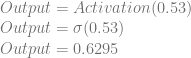
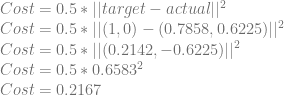
The neurons use the sigmoid activation function, and the cost function used is half mean squared error.
Training uses a learning rate of 3.0 and the training data is processed by the network 30 times (aka 30 training epochs), using a minibatch size of 10.
A minibatch size of 10 just means that we calculate the gradient for 10 training samples at a time and adjust the weights and biases using that gradient. We do that for the entire (shuffled) 60,000 training items and call that a single epoch. 30 epochs mean we do this full process 30 times.
There are 60,000 items in the training data, mapping 28×28 greyscale images to what digit 0-9 they actually represent.
Besides the 60,000 training data items, there are also 10,000 separate items that are the test data. These test data items are items never seen by the network during training and are just used as a way to see how well the network has learned about the problem in general, versus learning about the specific training data items.
The test and training data is the MNIST data set. I have a link to zip file I made with the data in it below, but this is where I got the data from: The MNIST database of handwritten digits.
That is the entire recipe!
Results
The 30 training epochs took 1 minute 22 seconds on my machine in release x64 (with REPORT_ERROR_WHILE_TRAINING() set to 0 to speed things up), but the code could be made to run faster by using SIMD, putting it on the GPU, getting multithreading involved or other things.
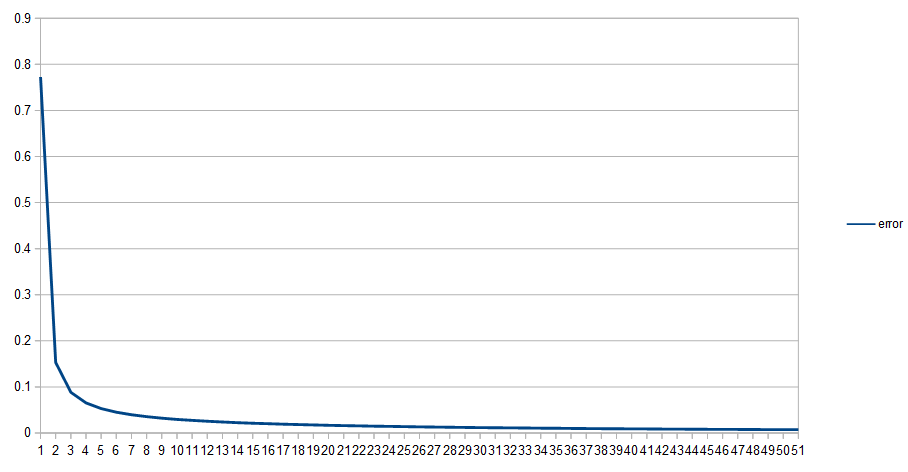
Below is a graph of the accuracy during the training epochs.
Notice that most learning happened very early on and then only slowly improved from there. This is due to our neuron activation functions and also our cost function. There are better choices for both, but this is also an ongoing area of research to improve in neural networks.
The end result of my training run is 95.32% accuracy but you may get slightly higher or lower due to random initialization of weights and biases. That sounds pretty high, but if you were actually using this, 4 or 5 numbers wrong out of 100 is a pretty big deal! The record for MNIST is 99.77% accuracy using “a committee of convolutional networks” where they distorted the input data during training to make it learn in a more generalized way (described as “committee of 35 conv. net, 1-20-P-40-P-150-10 [elastic distortions]”).
A better cost function would probably be the cross entropy cost function, a better activation function than sigmoid would probably be an ELU (Exponential Linear Unit). A soft max layer could be used instead of just taking the maximum output neuron as the answer. The weights could be initialized to smarter values. We could also use a convolutional layer to help let the network learn features in a way that didn’t also tie the features to specific locations in the images.
Many of these things are described in good detail at http://neuralnetworksanddeeplearning.com/, particularly in chapter 3 where they make a python implementation of a convolutional neural network which performs better than this one. I highly recommend checking that website out!
HTML5 Demo
You can play with a network created with this recipe here: Recognize Handwritten Digit 95% Accuracy
Here is an example of it correctly detecting that I drew a 4.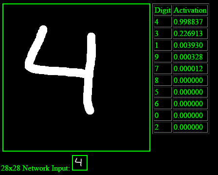
The demo works “pretty well” but it does have a little less than 95% accuracy.
The reason for this though is that it isn’t comparing apples to apples.
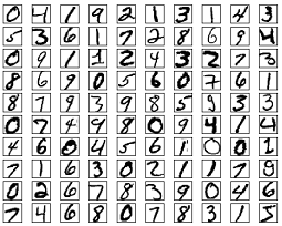
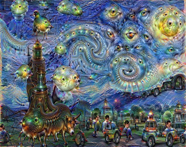
A handwritten digit isn’t quite the same as a digit drawn with a mouse. Check out the image below to see 100 of the training images and see what i mean.
The demo finds the bounding box of the drawn image and rescales that bounding box to a 20×20 image, preserving the aspect ratio. It then puts that into a 28×28 image, using the center of mass of the pixels to center the smaller image in the larger one. This is how the MNIST data was generated, so makes the demo more accurate, but it also has the nice side effect of making it so you can draw a number of any size, in any part of the box, and it will treat it the same as if you drew it at a difference size, or in a different part of the box.
The code that goes with this post outputs the weights, biases and network structure in a json format that is very easy to drop into the html5 demo. This way, if you want to try different things in the network, it should be fairly low effort to adjust the demo to try your adjustments there as well.
Lastly, it might be interesting to get the derivatives of the inputs and play around with the input you gave it. Some experiments I can think of:
- When it misclassifies what number you drew, have it adjust what you drew (the input) to be more like what the network would expect to see for that digit. This could help show why it misclassified your number.
- Start with a well classified number and make it morph into something recognized by the network as a different number.
- Start with a random static (noise) image and adjust it until the network recognizes it as a digit. It would be interesting to see if it looked anything like a number, or if it was still just static.
Source Code
The source code and mnist data is on github at MNIST1, but is also included below for your convenience.
If grabbing the source code from below instead of github, you will need to extract this zip file into the working directory of the program as well. It contains the test data used for training the network.
mnist.zip
Note: it’s been reported on that some compilers/OSs, std::random_device will use dev/urandom which can result in lower quality random numbers, which can result in the network not learning as quickly or to as high of accuracy. You can force it to use dev/random instead which will fix that problem. Details can be found here: http://en.cppreference.com/w/cpp/numeric/random/random_device/random_device
#define _CRT_SECURE_NO_WARNINGS
#include <stdio.h>
#include <stdint.h>
#include <stdlib.h>
#include <random>
#include <array>
#include <vector>
#include <algorithm>
#include <chrono>
typedef uint32_t uint32;
typedef uint16_t uint16;
typedef uint8_t uint8;
// Set to 1 to have it show error after each training and also writes it to an Error.csv file.
// Slows down the process a bit (+~50% time on my machine)
#define REPORT_ERROR_WHILE_TRAINING() 1
const size_t c_numInputNeurons = 784;
const size_t c_numHiddenNeurons = 30; // NOTE: setting this to 100 hidden neurons can give better results, but also can be worse other times.
const size_t c_numOutputNeurons = 10;
const size_t c_trainingEpochs = 30;
const size_t c_miniBatchSize = 10;
const float c_learningRate = 3.0f;
// ============================================================================================
// SBlockTimer
// ============================================================================================
// times a block of code
struct SBlockTimer
{
SBlockTimer (const char* label)
{
m_start = std::chrono::high_resolution_clock::now();
m_label = label;
}
~SBlockTimer ()
{
std::chrono::duration<float> seconds = std::chrono::high_resolution_clock::now() - m_start;
printf("%s%0.2f seconds\n", m_label, seconds.count());
}
std::chrono::high_resolution_clock::time_point m_start;
const char* m_label;
};
// ============================================================================================
// MNIST DATA LOADER
// ============================================================================================
inline uint32 EndianSwap (uint32 a)
{
return (a<<24) | ((a<<8) & 0x00ff0000) |
((a>>8) & 0x0000ff00) | (a>>24);
}
// MNIST data and file format description is from http://yann.lecun.com/exdb/mnist/
class CMNISTData
{
public:
CMNISTData ()
{
m_labelData = nullptr;
m_imageData = nullptr;
m_imageCount = 0;
m_labels = nullptr;
m_pixels = nullptr;
}
bool Load (bool training)
{
// set the expected image count
m_imageCount = training ? 60000 : 10000;
// read labels
const char* labelsFileName = training ? "train-labels.idx1-ubyte" : "t10k-labels.idx1-ubyte";
FILE* file = fopen(labelsFileName,"rb");
if (!file)
{
printf("could not open %s for reading.\n", labelsFileName);
return false;
}
fseek(file, 0, SEEK_END);
long fileSize = ftell(file);
fseek(file, 0, SEEK_SET);
m_labelData = new uint8[fileSize];
fread(m_labelData, fileSize, 1, file);
fclose(file);
// read images
const char* imagesFileName = training ? "train-images.idx3-ubyte" : "t10k-images.idx3-ubyte";
file = fopen(imagesFileName, "rb");
if (!file)
{
printf("could not open %s for reading.\n", imagesFileName);
return false;
}
fseek(file, 0, SEEK_END);
fileSize = ftell(file);
fseek(file, 0, SEEK_SET);
m_imageData = new uint8[fileSize];
fread(m_imageData, fileSize, 1, file);
fclose(file);
// endian swap label file if needed, just first two uint32's. The rest is uint8's.
uint32* data = (uint32*)m_labelData;
if (data[0] == 0x01080000)
{
data[0] = EndianSwap(data[0]);
data[1] = EndianSwap(data[1]);
}
// verify that the label file has the right header
if (data[0] != 2049 || data[1] != m_imageCount)
{
printf("Label data had unexpected header values.\n");
return false;
}
m_labels = (uint8*)&(data[2]);
// endian swap the image file if needed, just first 4 uint32's. The rest is uint8's.
data = (uint32*)m_imageData;
if (data[0] == 0x03080000)
{
data[0] = EndianSwap(data[0]);
data[1] = EndianSwap(data[1]);
data[2] = EndianSwap(data[2]);
data[3] = EndianSwap(data[3]);
}
// verify that the image file has the right header
if (data[0] != 2051 || data[1] != m_imageCount || data[2] != 28 || data[3] != 28)
{
printf("Label data had unexpected header values.\n");
return false;
}
m_pixels = (uint8*)&(data[4]);
// convert the pixels from uint8 to float
m_pixelsFloat.resize(28 * 28 * m_imageCount);
for (size_t i = 0; i < 28 * 28 * m_imageCount; ++i)
m_pixelsFloat[i] = float(m_pixels[i]) / 255.0f;
// success!
return true;
}
~CMNISTData ()
{
delete[] m_labelData;
delete[] m_imageData;
}
size_t NumImages () const { return m_imageCount; }
const float* GetImage (size_t index, uint8& label) const
{
label = m_labels[index];
return &m_pixelsFloat[index * 28 * 28];
}
private:
void* m_labelData;
void* m_imageData;
size_t m_imageCount;
uint8* m_labels;
uint8* m_pixels;
std::vector<float> m_pixelsFloat;
};
// ============================================================================================
// NEURAL NETWORK
// ============================================================================================
template <size_t INPUTS, size_t HIDDEN_NEURONS, size_t OUTPUT_NEURONS>
class CNeuralNetwork
{
public:
CNeuralNetwork ()
{
// initialize weights and biases to a gaussian distribution random number with mean 0, stddev 1.0
std::random_device rd;
std::mt19937 e2(rd());
std::normal_distribution<float> dist(0, 1);
for (float& f : m_hiddenLayerBiases)
f = dist(e2);
for (float& f : m_outputLayerBiases)
f = dist(e2);
for (float& f : m_hiddenLayerWeights)
f = dist(e2);
for (float& f : m_outputLayerWeights)
f = dist(e2);
}
void Train (const CMNISTData& trainingData, size_t miniBatchSize, float learningRate)
{
// shuffle the order of the training data for our mini batches
if (m_trainingOrder.size() != trainingData.NumImages())
{
m_trainingOrder.resize(trainingData.NumImages());
size_t index = 0;
for (size_t& v : m_trainingOrder)
{
v = index;
++index;
}
}
static std::random_device rd;
static std::mt19937 e2(rd());
std::shuffle(m_trainingOrder.begin(), m_trainingOrder.end(), e2);
// process all minibatches until we are out of training examples
size_t trainingIndex = 0;
while (trainingIndex < trainingData.NumImages())
{
// Clear out minibatch derivatives. We sum them up and then divide at the end of the minimatch
std::fill(m_miniBatchHiddenLayerBiasesDeltaCost.begin(), m_miniBatchHiddenLayerBiasesDeltaCost.end(), 0.0f);
std::fill(m_miniBatchOutputLayerBiasesDeltaCost.begin(), m_miniBatchOutputLayerBiasesDeltaCost.end(), 0.0f);
std::fill(m_miniBatchHiddenLayerWeightsDeltaCost.begin(), m_miniBatchHiddenLayerWeightsDeltaCost.end(), 0.0f);
std::fill(m_miniBatchOutputLayerWeightsDeltaCost.begin(), m_miniBatchOutputLayerWeightsDeltaCost.end(), 0.0f);
// process the minibatch
size_t miniBatchIndex = 0;
while (miniBatchIndex < miniBatchSize && trainingIndex < trainingData.NumImages())
{
// get the training item
uint8 imageLabel = 0;
const float* pixels = trainingData.GetImage(m_trainingOrder[trainingIndex], imageLabel);
// run the forward pass of the network
uint8 labelDetected = ForwardPass(pixels, imageLabel);
// run the backward pass to get derivatives of the cost function
BackwardPass(pixels, imageLabel);
// add the current derivatives into the minibatch derivative arrays so we can average them at the end of the minibatch via division.
for (size_t i = 0; i < m_hiddenLayerBiasesDeltaCost.size(); ++i)
m_miniBatchHiddenLayerBiasesDeltaCost[i] += m_hiddenLayerBiasesDeltaCost[i];
for (size_t i = 0; i < m_outputLayerBiasesDeltaCost.size(); ++i)
m_miniBatchOutputLayerBiasesDeltaCost[i] += m_outputLayerBiasesDeltaCost[i];
for (size_t i = 0; i < m_hiddenLayerWeightsDeltaCost.size(); ++i)
m_miniBatchHiddenLayerWeightsDeltaCost[i] += m_hiddenLayerWeightsDeltaCost[i];
for (size_t i = 0; i < m_outputLayerWeightsDeltaCost.size(); ++i)
m_miniBatchOutputLayerWeightsDeltaCost[i] += m_outputLayerWeightsDeltaCost[i];
// note that we've added another item to the minibatch, and that we've consumed another training example
++trainingIndex;
++miniBatchIndex;
}
// divide minibatch derivatives by how many items were in the minibatch, to get the average of the derivatives.
// NOTE: instead of doing this explicitly like in the commented code below, we'll do it implicitly
// by dividing the learning rate by miniBatchIndex.
/*
for (float& f : m_miniBatchHiddenLayerBiasesDeltaCost)
f /= float(miniBatchIndex);
for (float& f : m_miniBatchOutputLayerBiasesDeltaCost)
f /= float(miniBatchIndex);
for (float& f : m_miniBatchHiddenLayerWeightsDeltaCost)
f /= float(miniBatchIndex);
for (float& f : m_miniBatchOutputLayerWeightsDeltaCost)
f /= float(miniBatchIndex);
*/
float miniBatchLearningRate = learningRate / float(miniBatchIndex);
// apply training to biases and weights
for (size_t i = 0; i < m_hiddenLayerBiases.size(); ++i)
m_hiddenLayerBiases[i] -= m_miniBatchHiddenLayerBiasesDeltaCost[i] * miniBatchLearningRate;
for (size_t i = 0; i < m_outputLayerBiases.size(); ++i)
m_outputLayerBiases[i] -= m_miniBatchOutputLayerBiasesDeltaCost[i] * miniBatchLearningRate;
for (size_t i = 0; i < m_hiddenLayerWeights.size(); ++i)
m_hiddenLayerWeights[i] -= m_miniBatchHiddenLayerWeightsDeltaCost[i] * miniBatchLearningRate;
for (size_t i = 0; i < m_outputLayerWeights.size(); ++i)
m_outputLayerWeights[i] -= m_miniBatchOutputLayerWeightsDeltaCost[i] * miniBatchLearningRate;
}
}
// This function evaluates the network for the given input pixels and returns the label it thinks it is from 0-9
uint8 ForwardPass (const float* pixels, uint8 correctLabel)
{
// first do hidden layer
for (size_t neuronIndex = 0; neuronIndex < HIDDEN_NEURONS; ++neuronIndex)
{
float Z = m_hiddenLayerBiases[neuronIndex];
for (size_t inputIndex = 0; inputIndex < INPUTS; ++inputIndex)
Z += pixels[inputIndex] * m_hiddenLayerWeights[HiddenLayerWeightIndex(inputIndex, neuronIndex)];
m_hiddenLayerOutputs[neuronIndex] = 1.0f / (1.0f + std::exp(-Z));
}
// then do output layer
for (size_t neuronIndex = 0; neuronIndex < OUTPUT_NEURONS; ++neuronIndex)
{
float Z = m_outputLayerBiases[neuronIndex];
for (size_t inputIndex = 0; inputIndex < HIDDEN_NEURONS; ++inputIndex)
Z += m_hiddenLayerOutputs[inputIndex] * m_outputLayerWeights[OutputLayerWeightIndex(inputIndex, neuronIndex)];
m_outputLayerOutputs[neuronIndex] = 1.0f / (1.0f + std::exp(-Z));
}
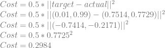
// calculate error.
// this is the magnitude of the vector that is Desired - Actual.
// Commenting out because it's not needed.
/*
{
error = 0.0f;
for (size_t neuronIndex = 0; neuronIndex < OUTPUT_NEURONS; ++neuronIndex)
{
float desiredOutput = (correctLabel == neuronIndex) ? 1.0f : 0.0f;
float diff = (desiredOutput - m_outputLayerOutputs[neuronIndex]);
error += diff * diff;
}
error = std::sqrt(error);
}
*/
// find the maximum value of the output layer and return that index as the label
float maxOutput = m_outputLayerOutputs[0];
uint8 maxLabel = 0;
for (uint8 neuronIndex = 1; neuronIndex < OUTPUT_NEURONS; ++neuronIndex)
{
if (m_outputLayerOutputs[neuronIndex] > maxOutput)
{
maxOutput = m_outputLayerOutputs[neuronIndex];
maxLabel = neuronIndex;
}
}
return maxLabel;
}
// Functions to get weights/bias values. Used to make the JSON file.
const std::array<float, HIDDEN_NEURONS>& GetHiddenLayerBiases () const { return m_hiddenLayerBiases; }
const std::array<float, OUTPUT_NEURONS>& GetOutputLayerBiases () const { return m_outputLayerBiases; }
const std::array<float, INPUTS * HIDDEN_NEURONS>& GetHiddenLayerWeights () const { return m_hiddenLayerWeights; }
const std::array<float, HIDDEN_NEURONS * OUTPUT_NEURONS>& GetOutputLayerWeights () const { return m_outputLayerWeights; }
private:
static size_t HiddenLayerWeightIndex (size_t inputIndex, size_t hiddenLayerNeuronIndex)
{
return hiddenLayerNeuronIndex * INPUTS + inputIndex;
}
static size_t OutputLayerWeightIndex (size_t hiddenLayerNeuronIndex, size_t outputLayerNeuronIndex)
{
return outputLayerNeuronIndex * HIDDEN_NEURONS + hiddenLayerNeuronIndex;
}
// this function uses the neuron output values from the forward pass to backpropagate the error
// of the network to calculate the gradient needed for training. It figures out what the error
// is by comparing the label it came up with to the label it should have come up with (correctLabel).
void BackwardPass (const float* pixels, uint8 correctLabel)
{
// since we are going backwards, do the output layer first
for (size_t neuronIndex = 0; neuronIndex < OUTPUT_NEURONS; ++neuronIndex)
{
// calculate deltaCost/deltaBias for each output neuron.
// This is also the error for the neuron, and is the same value as deltaCost/deltaZ.
//
// deltaCost/deltaZ = deltaCost/deltaO * deltaO/deltaZ
//
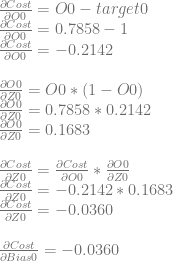
// deltaCost/deltaO = O - desiredOutput
// deltaO/deltaZ = O * (1 - O)
//
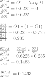
float desiredOutput = (correctLabel == neuronIndex) ? 1.0f : 0.0f;
float deltaCost_deltaO = m_outputLayerOutputs[neuronIndex] - desiredOutput;
float deltaO_deltaZ = m_outputLayerOutputs[neuronIndex] * (1.0f - m_outputLayerOutputs[neuronIndex]);
m_outputLayerBiasesDeltaCost[neuronIndex] = deltaCost_deltaO * deltaO_deltaZ;
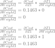
// calculate deltaCost/deltaWeight for each weight going into the neuron
//
// deltaCost/deltaWeight = deltaCost/deltaZ * deltaCost/deltaWeight
// deltaCost/deltaWeight = deltaCost/deltaBias * input
//
for (size_t inputIndex = 0; inputIndex < HIDDEN_NEURONS; ++inputIndex)
m_outputLayerWeightsDeltaCost[OutputLayerWeightIndex(inputIndex, neuronIndex)] = m_outputLayerBiasesDeltaCost[neuronIndex] * m_hiddenLayerOutputs[inputIndex];
}
// then do the hidden layer
for (size_t neuronIndex = 0; neuronIndex < HIDDEN_NEURONS; ++neuronIndex)
{
// calculate deltaCost/deltaBias for each hidden neuron.
// This is also the error for the neuron, and is the same value as deltaCost/deltaZ.
//
// deltaCost/deltaO =
// Sum for each output of this neuron:
// deltaCost/deltaDestinationZ * deltaDestinationZ/deltaSourceO
//
// deltaCost/deltaDestinationZ is already calculated and lives in m_outputLayerBiasesDeltaCost[destinationNeuronIndex].
// deltaTargetZ/deltaSourceO is the value of the weight connecting the source and target neuron.
//
// deltaCost/deltaZ = deltaCost/deltaO * deltaO/deltaZ
// deltaO/deltaZ = O * (1 - O)
//
float deltaCost_deltaO = 0.0f;
for (size_t destinationNeuronIndex = 0; destinationNeuronIndex < OUTPUT_NEURONS; ++destinationNeuronIndex)
deltaCost_deltaO += m_outputLayerBiasesDeltaCost[destinationNeuronIndex] * m_outputLayerWeights[OutputLayerWeightIndex(neuronIndex, destinationNeuronIndex)];
float deltaO_deltaZ = m_hiddenLayerOutputs[neuronIndex] * (1.0f - m_hiddenLayerOutputs[neuronIndex]);
m_hiddenLayerBiasesDeltaCost[neuronIndex] = deltaCost_deltaO * deltaO_deltaZ;
// calculate deltaCost/deltaWeight for each weight going into the neuron
//
// deltaCost/deltaWeight = deltaCost/deltaZ * deltaCost/deltaWeight
// deltaCost/deltaWeight = deltaCost/deltaBias * input
//
for (size_t inputIndex = 0; inputIndex < INPUTS; ++inputIndex)
m_hiddenLayerWeightsDeltaCost[HiddenLayerWeightIndex(inputIndex, neuronIndex)] = m_hiddenLayerBiasesDeltaCost[neuronIndex] * pixels[inputIndex];
}
}
private:
// biases and weights
std::array<float, HIDDEN_NEURONS> m_hiddenLayerBiases;
std::array<float, OUTPUT_NEURONS> m_outputLayerBiases;
std::array<float, INPUTS * HIDDEN_NEURONS> m_hiddenLayerWeights;
std::array<float, HIDDEN_NEURONS * OUTPUT_NEURONS> m_outputLayerWeights;
// neuron activation values aka "O" values
std::array<float, HIDDEN_NEURONS> m_hiddenLayerOutputs;
std::array<float, OUTPUT_NEURONS> m_outputLayerOutputs;
// derivatives of biases and weights for a single training example
std::array<float, HIDDEN_NEURONS> m_hiddenLayerBiasesDeltaCost;
std::array<float, OUTPUT_NEURONS> m_outputLayerBiasesDeltaCost;
std::array<float, INPUTS * HIDDEN_NEURONS> m_hiddenLayerWeightsDeltaCost;
std::array<float, HIDDEN_NEURONS * OUTPUT_NEURONS> m_outputLayerWeightsDeltaCost;
// derivatives of biases and weights for the minibatch. Average of all items in minibatch.
std::array<float, HIDDEN_NEURONS> m_miniBatchHiddenLayerBiasesDeltaCost;
std::array<float, OUTPUT_NEURONS> m_miniBatchOutputLayerBiasesDeltaCost;
std::array<float, INPUTS * HIDDEN_NEURONS> m_miniBatchHiddenLayerWeightsDeltaCost;
std::array<float, HIDDEN_NEURONS * OUTPUT_NEURONS> m_miniBatchOutputLayerWeightsDeltaCost;
// used for minibatch generation
std::vector<size_t> m_trainingOrder;
};
// ============================================================================================
// DRIVER PROGRAM
// ============================================================================================
// training and test data
CMNISTData g_trainingData;
CMNISTData g_testData;
// neural network
CNeuralNetwork<c_numInputNeurons, c_numHiddenNeurons, c_numOutputNeurons> g_neuralNetwork;
float GetDataAccuracy (const CMNISTData& data)
{
size_t correctItems = 0;
for (size_t i = 0, c = data.NumImages(); i < c; ++i)
{
uint8 label;
const float* pixels = data.GetImage(i, label);
uint8 detectedLabel = g_neuralNetwork.ForwardPass(pixels, label);
if (detectedLabel == label)
++correctItems;
}
return float(correctItems) / float(data.NumImages());
}
void ShowImage (const CMNISTData& data, size_t imageIndex)
{
uint8 label = 0;
const float* pixels = data.GetImage(imageIndex, label);
printf("showing a %i\n", label);
for (int iy = 0; iy < 28; ++iy)
{
for (int ix = 0; ix < 28; ++ix)
{
if (*pixels < 0.125)
printf(" ");
else
printf("+");
++pixels;
}
printf("\n");
}
}
int main (int argc, char** argv)
{
// load the MNIST data if we can
if (!g_trainingData.Load(true) || !g_testData.Load(false))
{
printf("Could not load mnist data, aborting!\n");
system("pause");
return 1;
}
#if REPORT_ERROR_WHILE_TRAINING()
FILE *file = fopen("Error.csv","w+t");
if (!file)
{
printf("Could not open Error.csv for writing, aborting!\n");
system("pause");
return 2;
}
fprintf(file, "\"Training Data Accuracy\",\"Testing Data Accuracy\"\n");
#endif
{
SBlockTimer timer("Training Time: ");
// train the network, reporting error before each training
for (size_t epoch = 0; epoch < c_trainingEpochs; ++epoch)
{
#if REPORT_ERROR_WHILE_TRAINING()
float accuracyTraining = GetDataAccuracy(g_trainingData);
float accuracyTest = GetDataAccuracy(g_testData);
printf("Training Data Accuracy: %0.2f%%\n", 100.0f*accuracyTraining);
printf("Test Data Accuracy: %0.2f%%\n\n", 100.0f*accuracyTest);
fprintf(file, "\"%f\",\"%f\"\n", accuracyTraining, accuracyTest);
#endif
printf("Training epoch %zu / %zu...\n", epoch+1, c_trainingEpochs);
g_neuralNetwork.Train(g_trainingData, c_miniBatchSize, c_learningRate);
printf("\n");
}
}
// report final error
float accuracyTraining = GetDataAccuracy(g_trainingData);
float accuracyTest = GetDataAccuracy(g_testData);
printf("\nFinal Training Data Accuracy: %0.2f%%\n", 100.0f*accuracyTraining);
printf("Final Test Data Accuracy: %0.2f%%\n\n", 100.0f*accuracyTest);
#if REPORT_ERROR_WHILE_TRAINING()
fprintf(file, "\"%f\",\"%f\"\n", accuracyTraining, accuracyTest);
fclose(file);
#endif
// Write out the final weights and biases as JSON for use in the web demo
{
FILE* file = fopen("WeightsBiasesJSON.txt", "w+t");
fprintf(file, "{\n");
// network structure
fprintf(file, " \"InputNeurons\":%zu,\n", c_numInputNeurons);
fprintf(file, " \"HiddenNeurons\":%zu,\n", c_numHiddenNeurons);
fprintf(file, " \"OutputNeurons\":%zu,\n", c_numOutputNeurons);
// HiddenBiases
auto hiddenBiases = g_neuralNetwork.GetHiddenLayerBiases();
fprintf(file, " \"HiddenBiases\" : [\n");
for (size_t i = 0; i < hiddenBiases.size(); ++i)
{
fprintf(file, " %f", hiddenBiases[i]);
if (i < hiddenBiases.size() -1)
fprintf(file, ",");
fprintf(file, "\n");
}
fprintf(file, " ],\n");
// HiddenWeights
auto hiddenWeights = g_neuralNetwork.GetHiddenLayerWeights();
fprintf(file, " \"HiddenWeights\" : [\n");
for (size_t i = 0; i < hiddenWeights.size(); ++i)
{
fprintf(file, " %f", hiddenWeights[i]);
if (i < hiddenWeights.size() - 1)
fprintf(file, ",");
fprintf(file, "\n");
}
fprintf(file, " ],\n");
// OutputBiases
auto outputBiases = g_neuralNetwork.GetOutputLayerBiases();
fprintf(file, " \"OutputBiases\" : [\n");
for (size_t i = 0; i < outputBiases.size(); ++i)
{
fprintf(file, " %f", outputBiases[i]);
if (i < outputBiases.size() - 1)
fprintf(file, ",");
fprintf(file, "\n");
}
fprintf(file, " ],\n");
// OutputWeights
auto outputWeights = g_neuralNetwork.GetOutputLayerWeights();
fprintf(file, " \"OutputWeights\" : [\n");
for (size_t i = 0; i < outputWeights.size(); ++i)
{
fprintf(file, " %f", outputWeights[i]);
if (i < outputWeights.size() - 1)
fprintf(file, ",");
fprintf(file, "\n");
}
fprintf(file, " ]\n");
// done
fprintf(file, "}\n");
fclose(file);
}
// You can use the code like the below to visualize an image if you want to.
//ShowImage(g_testData, 0);
system("pause");
return 0;
}
Thanks for reading, and if you have any questions, comments, or just want to chat, hit me up in the comments below, or on twitter at @Atrix256.


 and that the m value was the “rise over run” or the slope of the line. Well believe it or not, that’s all a derivative is. A derivative is just the slope of a function at a specific point on that function. Even if a function is curved, you can pick a point on the graph and get a slope at that point. The notation for a derivative is
  , which literally means “change in y divided by change in x”, or “delta y divided by delta x”, which is literally rise over run.
 .
. , you have two variables that you can take the derivative of. You can calculate
  and
and  . The first value tells you how much the z value changes for a change in x, the second value tells you how much the z value changes for a change in y.
 you have what is called the gradient vector.
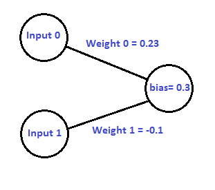
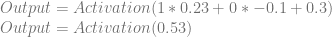
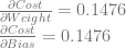
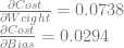
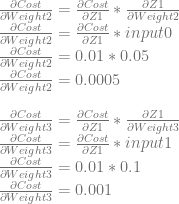
 , you would first calculate the cost of the network as usual, then you would add a small value to Weight0 and evaluate the cost again. You subtract the new cost from the old cost, and divide by the small value you added to Weight0. This will give you the partial derivative for that weight value. You’d repeat this for all your weights and biases.


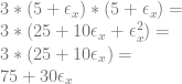
 , at input (5,2).

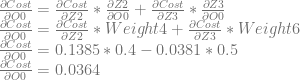
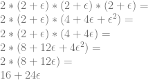
 value, keeping in mind that
  is zero:
 term:
term:
 term. We start by making our y value:

 value:


 term:
term:


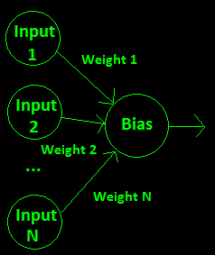
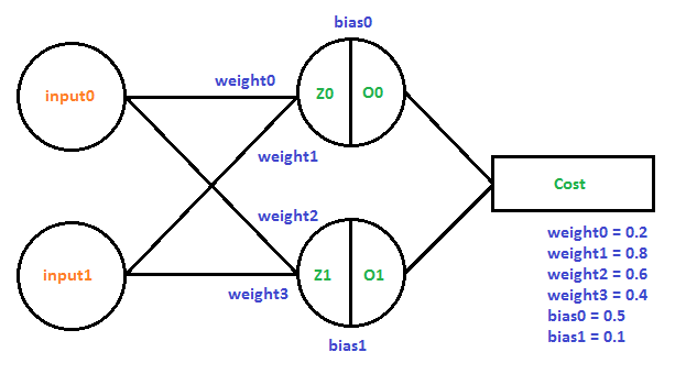
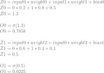
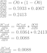
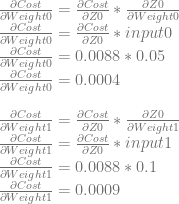
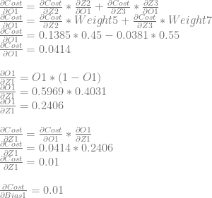
 is the bias,
  is the j’th weight and
  is the j’th input.