I talk and write a lot about noise so people will sometimes ask me about Perlin noise and other types of noise used for procedural content generation. I’m not usually much help because the noise I focus on is more about sampling and stochastic rendering techniques.

I was recently ray marching some Perlin noise based fog though, and came across Eevee’s (https://twitter.com/eevee) great write up on Perlin noise here: https://eev.ee/blog/2016/05/29/perlin-noise/

While reading that, it caught my eye that clumping of the random numbers was a problem. “Of course!” I thought to myself “White noise has clumping problems. I wonder how using blue noise instead would fare?” and decided to write this blog post, thinking also that low discrepancy sequences could be useful. This is the results of those and some more basic Perlin noise experiments. TL;DR nothing ground breaking was found, but there may still be some things of interest here.

The simple C++ code that generated the images for this post, and the small python script to make DFTs is available at https://github.com/Atrix256/Perlin.

Smoothing

2D Perlin noise uses a grid of 2D vectors that is smaller than the final image resolution. To shade a pixel, it gets the four corners of the cell containing the pixel, dot products the vector of each corner to the pixel with the vector at the corner, and does bilinear interpolation of this scalar value to get the color of the pixel.

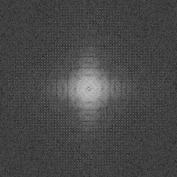
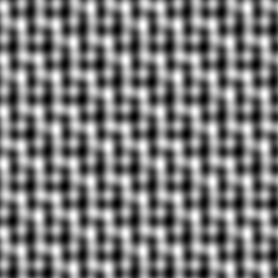
If you just do that, you get an image that looks like this (Image on left, discrete Fourier transform on right):

• 

• 

That obviously is no good, so just like Inigo Quilez does in his article (https://iquilezles.org/www/articles/texture/texture.htm), the fractional part of the pixel’s position on the grid is put through a smoothing function to round it out a bit. The original paper used smooth step (https://en.wikipedia.org/wiki/Smoothstep) which looks like this:

• 

• 

An improvement in a follow up paper is to use smoother step instead, which is a higher degree interpolating polynomial, which looks like this:

• 

• 

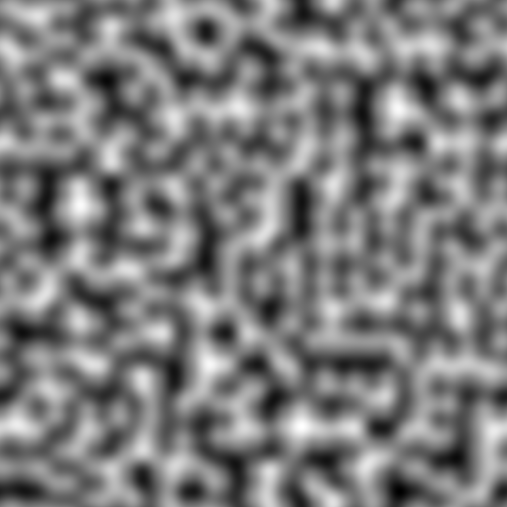
Different Sized Grids

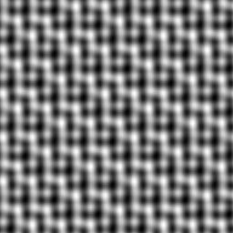
This shows what it looks like to use different sized grids for the perlin noise. The first uses 2×2 grids, then 4×4, then 8×8, then 16×16, then 32×32 and lastly 64×64. It’s interesting that the 2×2 grid Perlin noise looks a bit like blue noise. If you look at the DFT it does a bit as well, but is missing the highest frequencies at the corners, and has quite a bit of low frequency noise.

• 

• 

• 

• 

• 

• 

• 

• 

• 

• 

• 

• 

White Noise

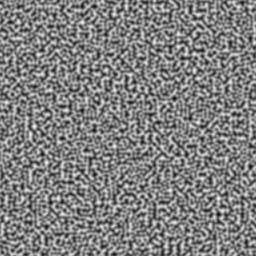
Here we use a cell size of 16×16 on 256×256 images, using 1, 2 and 3 octaves. Each octave uses the same (repeating) white noise vectors.

• 

• 

• 

• 

• 

• 

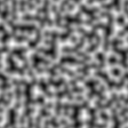
Here a different set of white noise vectors is used per octave, which doesn’t seem to change the quality much:

• 

• 

• 

• 

• 

• 

Blue Noise

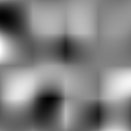
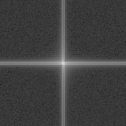
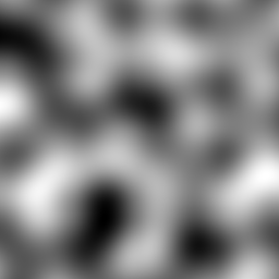
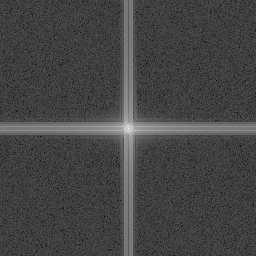
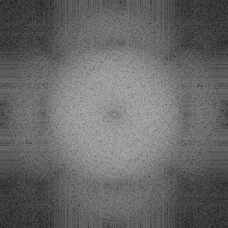
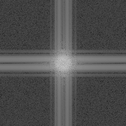
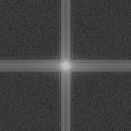
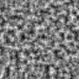
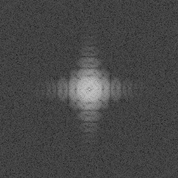
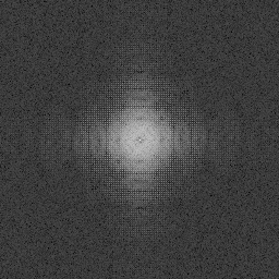
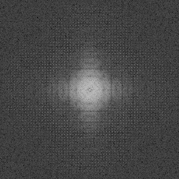
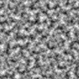
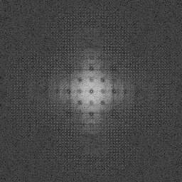
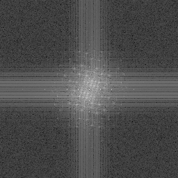
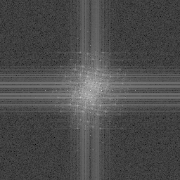
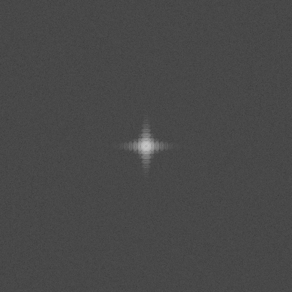
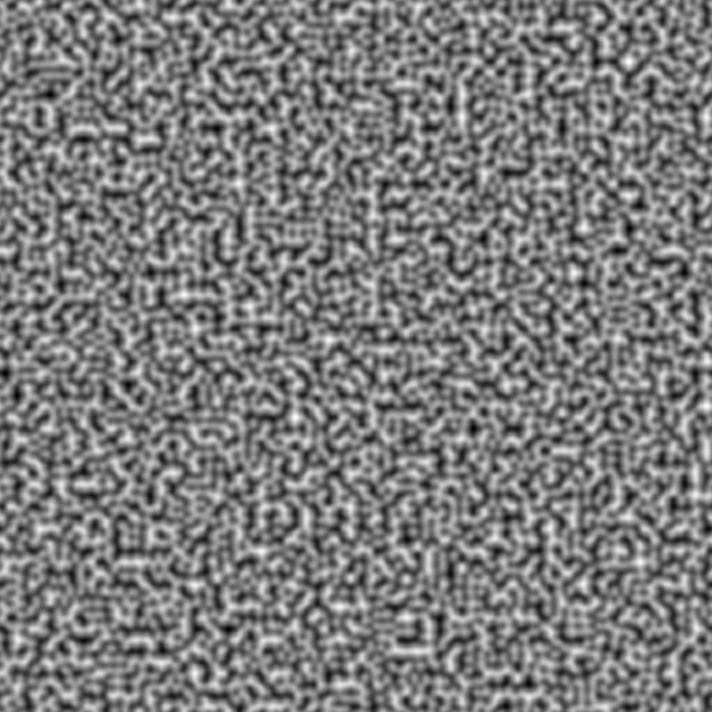
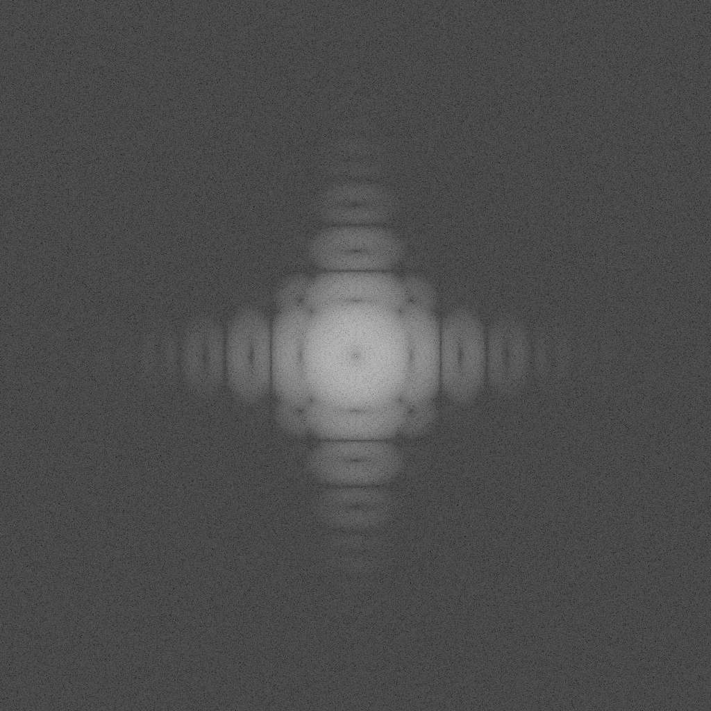
Here a 16×16 blue noise texture is used to generate the angle of the 2D vectors for the grid, on the 256×256 image. A 64×64 blue noise texture and DFT is also shown to see things more clearly. The same blue noise texture is used for each octave. First is the blue noise texture and DFT, then the Perlin noise made with 1, 2 and 3 octaves.

• 

• 

• 

• 

• 

• 

• 

• 

• 

• 

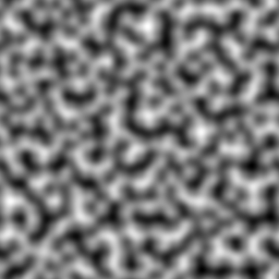
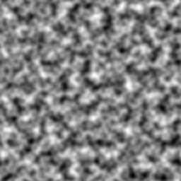
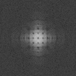
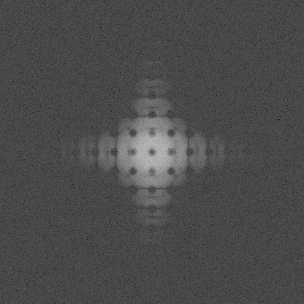
The noise doesn’t look that different visually when using blue noise instead of white, but the DFT has a bunch of dark circles repeated it in, which i believe is because the blue noise has a dark circle in the middle, and we are seeing some kind of convolutional effect. In any case, the lack of clumping in blue noise doesn’t seem to really change anything significantly.

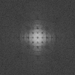
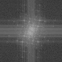
Here we use a “different” blue noise texture for each layer. We actually just use a low discrepancy sequence (R2 http://extremelearning.com.au/unreasonable-effectiveness-of-quasirandom-sequences/) to find an offset to read for each octave. Using an LDS to offset reads into a blue noise texture makes for roughly maximally independent reads, which can act as independent blue noise for some usage cases (not 100% sure if that’s true here since there are different scales of the same texture involved, but meh).

• 

• 

• 

• 

• 

• 

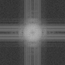
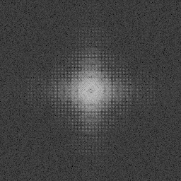
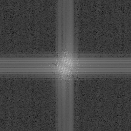
Interleaved Gradient Noise

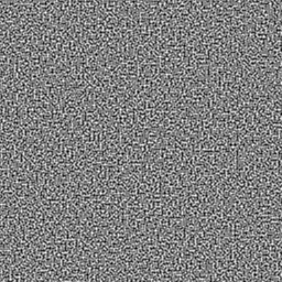
For the “low discrepancy sequence” route, we need a low discrepancy sequence which you plug in an 2D pixel integer index and get a scalar value out. I don’t know that common thinking calls IGN a low discrepancy sequence, or that something of this configuration could be considered a LDS, but I think of it as one because it has the property that every 3×3 block of values (even when they overlap!) have roughly all values 0/9, 1/9, … 8/9.

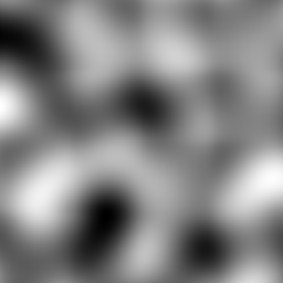
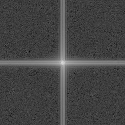
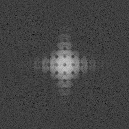
Here is IGN used to get the angle to make the vectors for the perlin noise grid, using the same noise values for each octave.

• 

• 

• 

• 

• 

• 

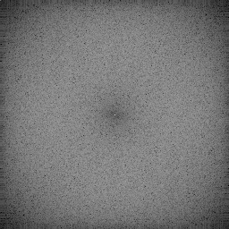
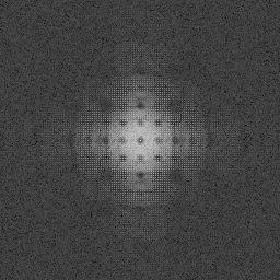
Here, R2 is used once again to make “independent” noise values per octave.

• 

• 

• 

• 

• 

• 

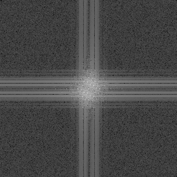
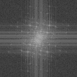
An interesting looking result but maybe not real useful. Maybe this just shows that you can plug different styles of noise into Perlin noise to get other looks in the results?

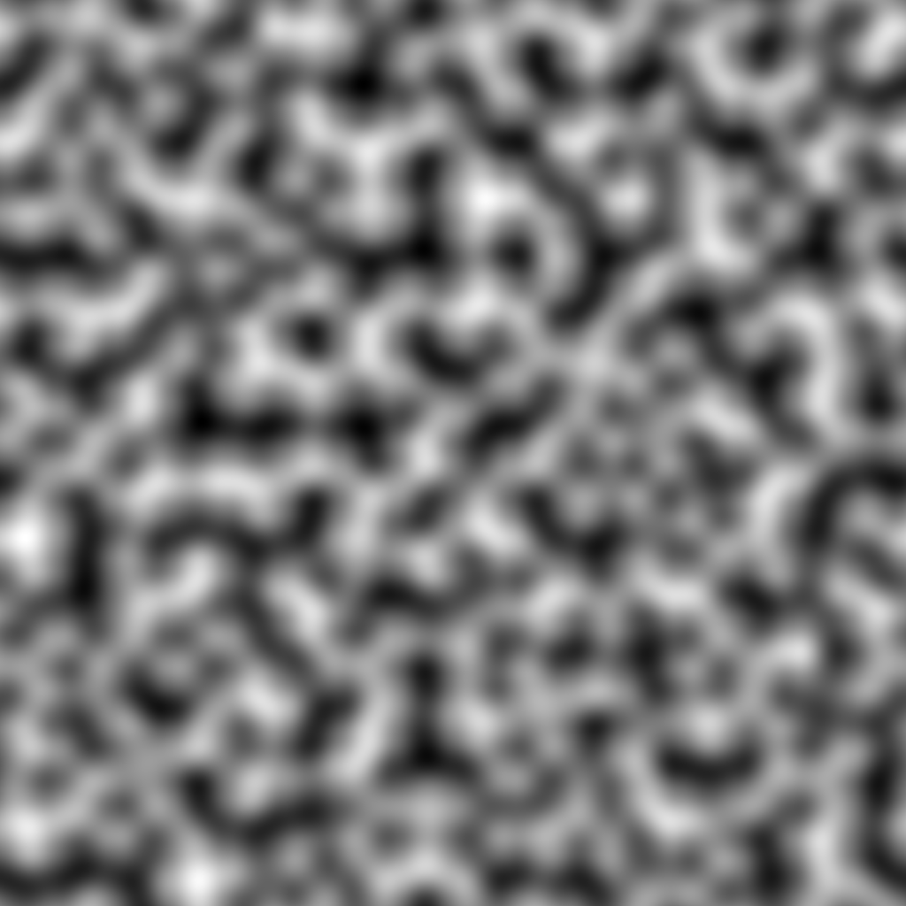
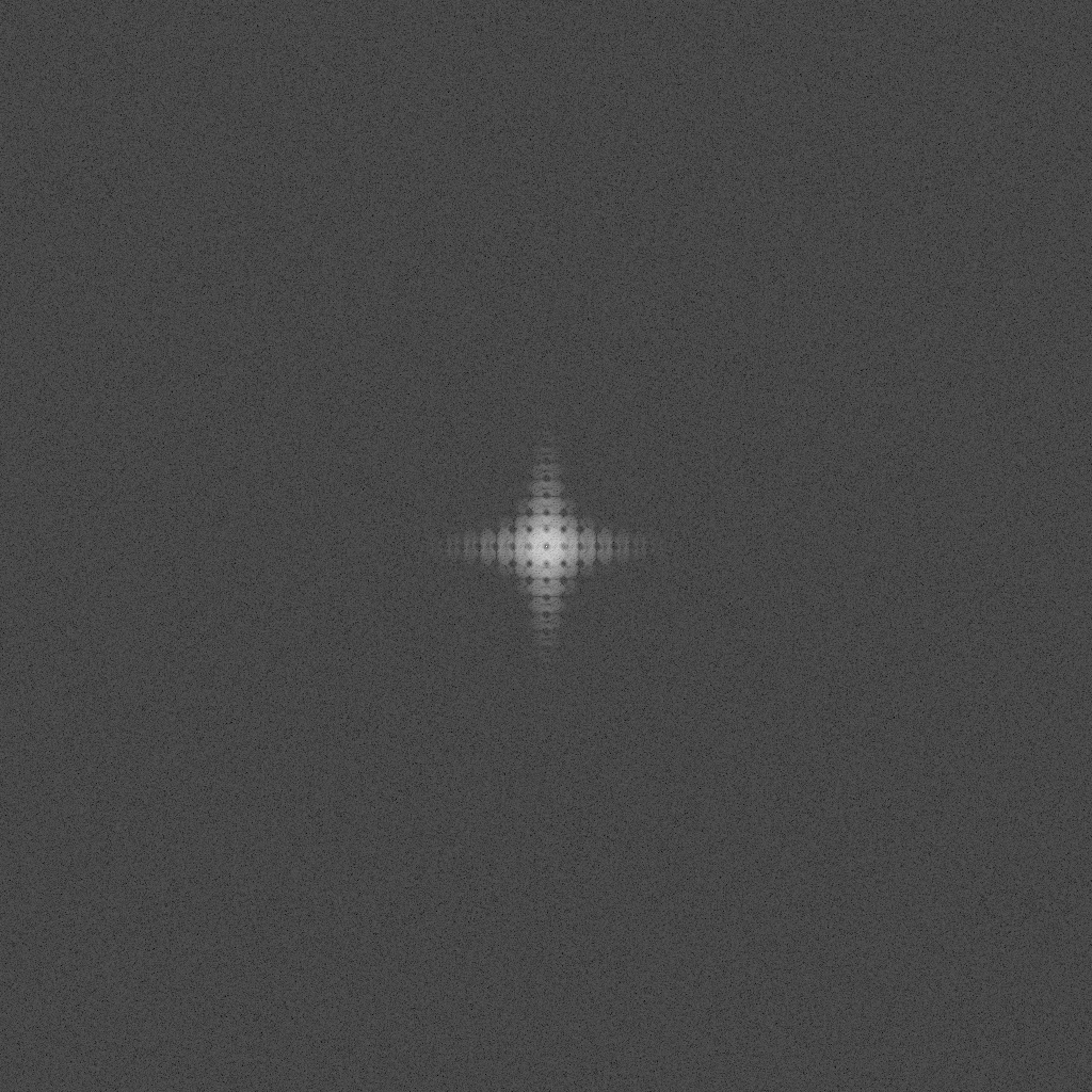
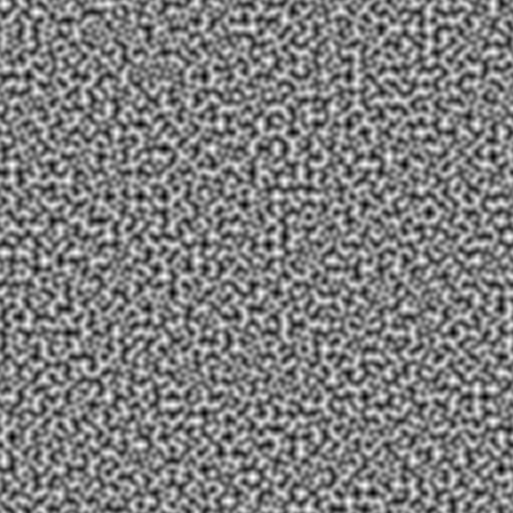
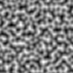
Bigger Renders

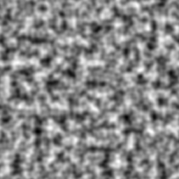
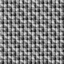
Here are larger renders of single octave white noise. First is a 16×16 grid, then a 64×64.

• 

• 

• 

• 

And here’s the same using blue noise – first the 16×16 blue noise texture used for the grid, then the 64×64 blue noise.

• 

• 

• 

• 

It’s April and this is my first blog post of the year. 2020/2021 has been a hard time for me like it has been for so many other people. After being absolutely destroyed at the end of last year, I discovered I have issues with both anxiety and depression and am talking to a therapist working through the problems, essentially debugging my life and thought patterns to live a better life. The virus and the BS related to the last president pushed me to a breaking point that I just couldn’t brute force muscle through like I normally do. Much improved now though luckily!

So, onto the main topic…

When analyzing randomized things, I often find myself wanting to graph averages to show how well things converge, and also wanting to graph variance or standard deviation to show how much they swing above and below that average. Averages alone can hide that important information. Variance shows up as noise when rendering too, so low variance is a nice thing.

I’ve seen quite a few sampling papers only report variance, not averages, and I never really understood why. The other day someone casually mentioned that mean squared error is variance and it threw me for a loop.

After thinking about it a bit, I was convinced: mean squared error is in fact variance, and root mean squared error is standard deviation. Let me show you…

To calculate the variance of a stream of values, you keep track of:

1. Average value
2. Average squared value

Then, variance is just this:

Variance = AverageSquaredValue – AverageValue*AverageValue

And you can square root that to get the standard deviation.

(Which BTW, there is a nice and easy numerically stable way to keep a “running average” that you can read about here: https://blog.demofox.org/2016/08/23/incremental-averaging/)

When we are talking about error, we know that the average value should be 0 if our process is unbiased, so we can modify the variance equation to be the below:

Variance = AverageSquaredValue

And since the value we are tracking is error, we can write it as:

Variance = AverageSquaredError

MSE is “mean squared error” where the word average above is the mean, so…

Variance = MeanSquaredError

And you can square root that to get the standard deviation of the error, which is also RMSE “Root Mean Squared Error”.

The nice thing about MSE being variance and RMSE being std dev is that if you are ok seeing squared error instead of regular error, you can have a single graph that communicates both error and variance in one.

I also find it interesting that squared error is used because that links it to “least squares” curve fitting (https://blog.demofox.org/2016/12/22/incremental-least-squares-curve-fitting/), which is pretty darn useful, and makes it feel a lot more ok to be looking at squared error instead of regular error. A benefit of using squared error is that it makes outliers a lot larger / more costly. This means that given the choice between one large error, or many little ones that equal the same amount of error, it will choose the many little ones instead. That means less noise in a render, and less variance.

This was a short post, but I have another one in mind I want to write next – and soon – that ought to be pretty interesting, combining my favorite noise for sampling (blue noise) and a commonly used noise for procedural content generation (Perlin noise).

Until then, stay safe!