An Idea: Raytracing Lookup Tables

In rasterized rendering, one of the primary tools we have at our disposal is textures.

We use textures to store things like normal maps, roughness maps, pre-integrated lighting, and more.

We can even abuse the texture interpolator to evaluate arbitrary polynomials when the texture contains coefficients from the Bernstein Basis form of the polynomial (https://blog.demofox.org/2016/02/22/gpu-texture-sampler-bezier-curve-evaluation/).

In raytracing, we do still have the ability to use textures, and we will surely use them in fun new ways with the directx ray tracing support that was recently announced, but raytracing also gives us a different kind of tool: queryable geometry that doesn’t necessarily have to have any correlation to what actually shows up on screen.

This can be used for obvious things like soft shadows, reflections, volumetric lights, rendering non triangle based geometry (when doing procedural shapes), but it can be used for off label things too, just as we use textures for things other than putting color directly onto triangles.

Lookup Tables

One way I mentioned that textures are (ab)used is for making lookup tables for functions (pre-integrating lighting, the famous PBR split sum texture, etc).

A nice thing about using textures is that bilinear texture sampling is not very expensive on modern hardware compared to point sampling. This means that we can store data at whatever resolution we are ok with getting linear interpolation between.

GPUs interpolate in fixed point with 8 bits for fractional pixels, so the interpolation does break down at a point, but it is still really nice to get interpolated data values cheaply.

A not so nice thing about using textures for lookup tables is that texture data is stored in a regular grid, so you need to make the texture high enough resolution for the most demanding (high frequency) part of the data, while wasting higher resolution on the parts of your data that don’t need it.

Imagine that you have some function z=f(x,y) that you are trying to make a lookup table for. Let’s say that this data is nearly linear in almost all the places you care about, but that there is a very important, smaller section that has a curved part, where getting the curve right is very important to your results.

You’d have to use a high resolution texture to make sure the curved section was well represented, but the other parts would have much higher resolution than needed to represent them which is wasteful to memory and loading time.

(Devil’s advocate: you could address this by warping the uv space!)

Raytracing doesn’t have this problem however because you make a mesh of the function. (Or do you make a mess of the function? Only time will tell I guess!)

In your mesh, the z component of every vertex is the value f(x,y), and it’s up to you which (x,y) values to store. This is in direct contrast to a texture, where the (x,y) values are decided for you and are on a fixed grid.

For the specific function we mentioned, you could use only a few vertices in the places that were linear, and use a lot more vertices in the curved section. How many vertices to use is entirely up to you based on your quality, performance, and memory usage desired.

To actually get a value of this function out for a specific (x,y), assuming the function was always positive, you could cast a ray at the mesh from the position (x,y,0) in the direction (0,0,1). The time t of the ray intersection with the mesh is the value of z at f(x,y).

Something nice here is that you still get linear interpolation, like in the texture case, since a ray vs triangle test does a linear interpolation between the points on the triangle, using barycentric coordinates.

Something else nice is that when you get your intersection information from the ray vs triangle test, you will likely have access to the barycentric coordinates of the intersection, as well as per vertex data. This means that you could store other information per vertex and get a linearly interpolated result, including the data from other functions with entirely different shapes.

This is one way to get around the fact that a texture lookup can give you multiple values as a result (RGBA), while a raytraced lookup can only give you one (ray intersection time) with a naive implementation.

This also lets you do a SIMD type thing, where if you have N functions you are always going to look up for the same input values (Think: diffuse and specular term of image based lighting), that you can do one raytrace to get the answer for all queries.

The “single value result” where you get only a time t ought to be more performant than the multiple value result where you (manually) interpolate vertex data, but as vertex data interpolation is the common case for using the raytracing API, i wouldn’t expect it to be unusably slow for a reasonable amount of data.

To make things really clear and explicit, you could literally replace a cubemap texture lookup with a raytrace into a scene instead, using the same direction vector (of course!). The time down the ray that the intersection happens would be the value of your cube map lookup in that direction. Since that’s only a single value, you could encode more values per triangle vertex and use the barycentric triangle interpolation to get the other values as well. This all works exactly like a texture lookup works, except you get to define your data set sparse in some areas, and dense in others. You are suddenly in control of your data sampling across the entire domain of your data!

When Should We Actually Do This?

So I don’t actually know how the performance of something like this would be on modern video cards – let alone future ones that are more geared to raytracing.

Experiments should be done to see if it can ever be faster than textures, use less memory than textures, or give higher quality than textures, and by how much under what circumstances.

How I’ve laid this out is just one of many ways to make a ray based lookup table, each with their own pros and cons.

For instance, if you have some hemispherical function z=f(x,y) where x and y are azimuth and altitude, the linear interpolation offered by this setup won’t be that great because the function is laid out like a heightfield, when the data really is hemispherical in nature.

If you instead changed the geometry to literally be a hemisphere that has points pushed in and pulled out, and you convert the angular coordinates to cartesian (a normalized direction vector) before the lookup, the linear interpolation offered by the intersection tests is going to be a lot friendlier to your data set.

I also wonder if there are better ray tracing acceleration structures than a generic solve (BVH with surface area heuristic?), when you intend to use the geo as a lookup table. I feel like knowing that the ray will always be vertical from the z=0 plane is important knowledge that could be used to make a better data structure. A grid based solution sure sounds decent (which ironically is how a texture works).

Anyhow, a total random idea I wanted to share.

There’s a forked twitter thread on these ideas and more here:

If you try this and get any details of perf, quality, mem use, etc please share here or hit me up on twitter at https://twitter.com/Atrix256.

Also, any other crazy raytracing ideas, i’d love to hear them (:

A Very Quick DirectX Raytracing API Primer

A raytracing API has been announced for DirectX and it seems like real time raytracing may finally be here?

MSDN: Announcing Microsoft DirectX Raytracing!
https://blogs.msdn.microsoft.com/directx/2018/03/19/announcing-microsoft-directx-raytracing/

How & where to get the new (experimental) SDK
http://forums.directxtech.com/index.php?topic=5860.0

There is some nice documentation in the SDK zip file, in the doc folder.

I’ve been lucky enough to be in a position to have played with it for a little while pre-release (about 1-2 weeks of time total) and it is pretty fun.

I’ve been playing with it from a purely triangle mesh perspective (don’t hate me! I know, I know…) and it seems like a hybrid rasterization / raytracing is the most realistic way to go there – eg, primary rays are rasterized, and maybe you do some rasterization style post processing. You actually don’t lose a whole lot going this way if you get creative. For instance, you could ray trace primary rays for non triangle based geo and take the minimum between that intersection time and the rasterized one. The only thing I feel like you lose is the ability to have the rays themselves deviate from a typical frustum setup, since you can’t really “distort rays” very easily while rasterizing.

However, I believe when looking at things from a non triangle based approach, things may be very different, especially on the performance side (better perf!). I would love to explore it myself, and know that many folks will also be exploring it. (I’m looking at you folks at the intersection of the twitter and shadertoy communities!)

Here is a very rough overview of some concepts of the Microsoft DirectX ray tracing API to help you form a mental model before trying to parse the verbose DX12 code. (It is DX12 only sadly!)

There are (useful) details missing for sure, but hopefully no misinformation. Please correct me if you see any (:

Raytracing acceleration structures:

  • Bottom Level Acceleration Structure – This is a “per object” acceleration structure. It can either be made from a triangle mesh, or you can specify that it’s a procedural shape. If it’s a procedural shape, you provide a bounding box and an intersection shader. The procedural shape will be useful for raymarching and other non triangle based ray-geometry intersection techniques.
  • Top Level Acceleration Structure – This is a “scene” acceleration structure. It contains instances of bottom level acceleration structures, each able to have their own instance data (like a transformation matrix).
  • Unfortunately the acceleration structures are made at runtime, and cannot be cached off to disk or similar. It’s a loading time cost that currently is seemingly unavoidable.

There are a few different types of shaders used for raytracing:

  • Ray Generation – This generates the primary rays. You could think of this like a compute shader that you author and run once per pixel. It’s also possible to do things like invoke it for each 2×2 pixel group in case you wanted to be able to have derivatives like when rasterizing. You call TraceRay() for each ray you want to generate, and you can use the results however you see fit. It’s typical you’d write the results to a texture or uav though. Whenever you call TraceRay(), you can provide payload data which can be read from and written to by the other shaders. This is useful for sending parameters down with the ray, or having other shaders return information like integrated fog density.
  • Any hit – Optional. As a ray traverses the acceleration structure, it will test objects in an order that is likely not front to back. You can supply an “any hit” shader that gets called during this process. You can read or write payload data in this shader, and you can also tell it to ignore a hit (useful for if you are doing alpha testing from a texture) or you can tell it to accept a hit and stop looking for other hits (useful perhaps for shadow rays). If you omit this shader, the hardware/software can make more assumptions about the ray traversal though and possibly run more quickly. So, you should only use it when necessary. You have access to barycentric information if intersecting with a triangle, and the triangle (index) itself. I’m unsure what you get in the procedural case.
  • Closest Hit – Optional. Called with the information about the closest hit. Called after all “any hit” shaders have been invoked. You have access to barycentric information if intersecting with a triangle, and the triangle (index) itself. I’m unsure what you get in the procedural case. You can call TraceRay() from this shader to spawn secondary rays.
  • Miss – Optional. Called if there are no hits for a ray. You could set some fog density to MAX_FLT, or could perhaps use this for shadow rays, assuming that there was a hit unless a miss shader was invoked.
    You can call TraceRay() from this shader to spawn secondary rays.
  • Yes, ray shaders can be recursive! a closest hit shader could spawn 3 rays which then have a closest hit which each spawn one more ray. There is a maximum stack depth, but recursive rays are totally supported.

When calling TraceRay() to shoot a ray out, you can give parameters such as…

  • Telling it to accept the first hit and end the search (useful for shadows)
  • Telling it to only test “opaque” geometry (anything that doesn’t have an any hit shaders)
  • Instance Masking – Each geometry instance can have an 8 bit mask. When you shoot a ray out, you can give an 8 bit mask that is ANDed with that instance mask, and will only consider geometry for intersection if the result is non zero. This is a bit like a stencil buffer.
  • A minimum and maximum time allowed for collision down the ray. This lets you ignore self intersection of secondary rays by setting the minimum to be greater than zero. The maximum time is useful for things like when shooting shadow rays at point light sources, to make sure you stop searching for occluding geometry at the light source.

There is the concept of a “Hit Group” which contains 0 or 1 of each shader type: intersection, any hit, closest hit.

You can specify a hit group per instance in the top level acceleration structure.

An intersection shader MUST be given for procedural geometry and MUST NOT be given for triangle based geometry.

If a shader is not specified on a hit group, it falls back to a default shader of each type that you specify. This is how you can make it so some objects have different behaviors than others for ray intersection / traversal etc.

You can also specify tables of shaders where shaders are accessible via indexing. This lets you pass numbers around to use in calculations for shader table indexing. In effect, this gives you the ability to have “function pointers” of shaders, and can even be exploited for non raytracing uses wherever having function pointers in shaders would be useful.

Lastly, this is something not super obvious when starting on raytracing, but sampling a mip mapped texture is a bit of a challenge because you no longer have automatic screen space derivatives of uv’s!

I’m sure good solutions to this will spread over time as more people dive into this raytracing API, but I personally think a good place to start is here:

Tracing Ray Differentials
http://graphics.stanford.edu/papers/trd/

That’s all for now! Anything small items think I should add, hit me up here or on twitter at https://twitter.com/Atrix256

Happy Raytracing Folks!! (:

Dissecting “Tiny Clouds”

There is an amazing shadertoy called “Tiny Clouds” by stubbe (twitter: @Stubbesaurus) which flies you through nearly photorealistic clouds in only 10 lines of code / 280 characters (2 old sized tweets or 1 new larger sized tweet).

The code is a bit dense, so I wanted to take some time to understand it and share the explanation for anyone else who was interested. Rune (the author) kindly answered a couple questions for me as well. Thanks Rune!

Link: [SH17A] Tiny Clouds (Check out this link, it looks even more amazing in motion)

Here is the code in full. The texture in iChannel0 is just a white noise texture that is bilinearly sampled.

#define T texture(iChannel0,(s*p.zw+ceil(s*p.x))/2e2).y/(s+=s)*4.
void mainImage(out vec4 O,vec2 x){
    vec4 p,d=vec4(.8,0,x/iResolution.y-.8),c=vec4(.6,.7,d);
    O=c-d.w;
    for(float f,s,t=2e2+sin(dot(x,x));--t>0.;p=.05*t*d)
        p.xz+=iTime,
        s=2.,
        f=p.w+1.-T-T-T-T,
    	f<0.?O+=(O-1.-f*c.zyxw)*f*.4:O;
}

BTW this shadertoy is a shrunken & reinterpreted version of a larger, more feature rich shadertoy by iq: Clouds

Before diving into the details of the code, here is how it works in short:

  • Every pixel does a ray march from far to near. It does it backwards to make for simpler alpha blending math.
  • At every ray step, it samples FBM data (fractal brownian motion) to figure out if the current position is below the surface of the cloud or above it.
  • If below, it alpha blends the pixel color with the cloud color at that point, using the vertical distance into the cloud as the cloud density.

Pretty reasonable and simple – and it would have to be, to look so good in so few characters! Let’s dig into the code.

#define T texture(iChannel0,(s*p.zw+ceil(s*p.x))/2e2).y/(s+=s)*4.
void mainImage(out vec4 O,vec2 x){
    vec4 p,d=vec4(.8,0,x/iResolution.y-.8),c=vec4(.6,.7,d);
    O=c-d.w;
    for(float f,s,t=2e2+sin(dot(x,x));--t>0.;p=.05*t*d)
        p.xz+=iTime,
        s=2.,
        f=p.w+1.-T-T-T-T,
    	f<0.?O+=(O-1.-f*c.zyxw)*f*.4:O;
}

Line 1 is a define that we’ll come back to and line 2 is just a minimal definition of the mainImage function.

#define T texture(iChannel0,(s*p.zw+ceil(s*p.x))/2e2).y/(s+=s)*4.
void mainImage(out vec4 O,vec2 x){
    vec4 p,d=vec4(.8,0,x/iResolution.y-.8),c=vec4(.6,.7,d);
    O=c-d.w;
    for(float f,s,t=2e2+sin(dot(x,x));--t>0.;p=.05*t*d)
        p.xz+=iTime,
        s=2.,
        f=p.w+1.-T-T-T-T,
    	f<0.?O+=(O-1.-f*c.zyxw)*f*.4:O;
}

On line 3 several variables are declared:

  • p – this is the variable that holds the position of the ray during the ray march. It isn’t initialized here, but that’s ok because the position is calculated each step in the loop. It is interesting to see that the y component of p is never used. p.x is actually depth into the screen, p.z is the screen x axis, and p.w is the screen y axis (aka the up axis). I believe that the axis choices and the fact that the y component is never used is purely to make the code smaller.
  • d – this is the direction that the ray for this pixel travels in. It uses the same axis conventions as p, and the y component is also never used (except implicitly for calculating p.y, which is never used). 0.8 is subtracted from d.z and d.w (the screen x and screen y axes). Interestingly that makes the screen x axis 0 nearly centered on the screen. It also points the screen y axis downward a bit, putting the 0 value near the top of the screen to make the camera look more downward at the clouds.
  • c – this is the color of the sky, which is a nice sky blue. It’s initialized with constants in x and y, and then d is used for z and w. d.xy goes into c.zw. That gives c the 0.8 value in the z field. I’m sure it was done this way because it’s fewer characters to initialize using “d” compared to “.8,0.” for the same effect. Note that c.w is used to calculate O.w (O.a) but that the alpha channel of the output pixel value is currently ignored by shadertoy, so this is a meaningless by product of the code, not a desired feature.
#define T texture(iChannel0,(s*p.zw+ceil(s*p.x))/2e2).y/(s+=s)*4.
void mainImage(out vec4 O,vec2 x){
    vec4 p,d=vec4(.8,0,x/iResolution.y-.8),c=vec4(.6,.7,d);
    O=c-d.w;
    for(float f,s,t=2e2+sin(dot(x,x));--t>0.;p=.05*t*d)
        p.xz+=iTime,
        s=2.,
        f=p.w+1.-T-T-T-T,
    	f<0.?O+=(O-1.-f*c.zyxw)*f*.4:O;
}

Line 4 initializes the output pixel color to be the sky color (c), but then subtracts d.w which is the pixel’s ray march direction on the screen y axis. This has a nice effect of making a nice sky blue gradient.

To see this in action, here we set O to c:

Here we set O to c-d.w:

It gets darker blue towards the top – where d.w is positive – because a positive number is being subtracted from the sky color. The color values get smaller.

It gets lighter towards the bottom – where d.w is negative – because a negative number is being subtracted from the sky color. The color values get larger.

#define T texture(iChannel0,(s*p.zw+ceil(s*p.x))/2e2).y/(s+=s)*4.
void mainImage(out vec4 O,vec2 x){
    vec4 p,d=vec4(.8,0,x/iResolution.y-.8),c=vec4(.6,.7,d);
    O=c-d.w;
    for(float f,s,t=2e2+sin(dot(x,x));--t>0.;p=.05*t*d)
        p.xz+=iTime,
        s=2.,
        f=p.w+1.-T-T-T-T,
    	f<0.?O+=(O-1.-f*c.zyxw)*f*.4:O;
}

On line 5, the for loop for ray marching starts. A few things happen here:

  • f is declared – f is the signed vertical distance from the current point in space to the cloud. If negative, it means that the point is inside the cloud. If positive, it means that the point is outside (above) the cloud. It isn’t initialized here, but it’s calculated each iteration of the loop so that’s fine.
  • s is declared – s is a scale value for use with the FBM data. FBMs work by sampling multiple octaves of data. You scale up the position and scale down the value for each octave. s is that scale value, used for both purposes. This isn’t initialized but is calculated each frame so that’s fine.
  • t is declared and initialized – t (aka ray march step index) is initialized to 2e2 aka 200. It was done this way because “2e2” is smaller than “200.” by one character. Note that the for loop takes t from 200 to 0. The ray marching happens back to front to simplify alpha blending. The sin(dot(x,x)) part I want to talk about briefly below.
  • p is calculated – p (aka the position in the current step of the ray march) is calculated, and this happens every step of the loop. p is t (time) multiplied by the direction of the ray for this pixel, and multiplied by .05 to scale it down.

The reason that sin(dot(x,x)) is added to the “ray time” is because the ray is marching through voxelized data (boxes). Unlike boxes, clouds are supposed to look organic, and not geometric. A way to fight the problem of the data looking boxy is to add a little noise to each ray to break up the geometric pattern. You can either literally add some noise to the result, or do what this shader does, which is add some noise to the starting position of the ray so that neighboring rays will cross the box (voxel) boundaries at different times and will look noisy instead of geometric.

I can’t see a difference when removing this from the shader, and other people have said the same. Rune says in the comments that it’d be on the chopping block for sure if he needed to shave off some more characters. He reached his 280 character goal, so no there is no need to remove it.

For what it’s worth, here is that expression visualized in the blue channel. the -1 to +1 is mapped to 0 to 1 by multiplying it by a half and adding a half:

#define T texture(iChannel0,(s*p.zw+ceil(s*p.x))/2e2).y/(s+=s)*4.
void mainImage(out vec4 O,vec2 x){
    vec4 p,d=vec4(.8,0,x/iResolution.y-.8),c=vec4(.6,.7,d);
    O=c-d.w;
    for(float f,s,t=2e2+sin(dot(x,x));--t>0.;p=.05*t*d)
        p.xz+=iTime,
        s=2.,
        f=p.w+1.-T-T-T-T,
    	f<0.?O+=(O-1.-f*c.zyxw)*f*.4:O;
}

Line 6 adds the current time to p.x and p.z. Remember that the x component is the axis pointing into the screen and the z component is the screen space x axis, so this line of code moves the camera forward and to the right over time.

If you are wondering why the lines in the for loop end in a comma instead of a semicolon, the reason is because if a semicolon was used instead, the for loop would require two more characters: “{” and “}” to show where the scope of the loop started and ended. Ending the lines with commas mean it’s one long statement, so the single line version of a for loop can be used. An interesting trick 😛

#define T texture(iChannel0,(s*p.zw+ceil(s*p.x))/2e2).y/(s+=s)*4.
void mainImage(out vec4 O,vec2 x){
    vec4 p,d=vec4(.8,0,x/iResolution.y-.8),c=vec4(.6,.7,d);
    O=c-d.w;
    for(float f,s,t=2e2+sin(dot(x,x));--t>0.;p=.05*t*d)
        p.xz+=iTime,
        s=2.,
        f=p.w+1.-T-T-T-T,
    	f<0.?O+=(O-1.-f*c.zyxw)*f*.4:O;
}

Line 7 sets / initializes s to 2. Remember that s is used as the octave scale for sample position and resulting value. That will come into play in the next line.

#define T texture(iChannel0,(s*p.zw+ceil(s*p.x))/2e2).y/(s+=s)*4.
void mainImage(out vec4 O,vec2 x){
    vec4 p,d=vec4(.8,0,x/iResolution.y-.8),c=vec4(.6,.7,d);
    O=c-d.w;
    for(float f,s,t=2e2+sin(dot(x,x));--t>0.;p=.05*t*d)
        p.xz+=iTime,
        s=2.,
        f=p.w+1.-T-T-T-T,
    	f<0.?O+=(O-1.-f*c.zyxw)*f*.4:O;
}

First let’s look at line 1, which is the “T” macro.

That macro samples the texture (which is just white noise) at a position described by the current ray position in the ray march. the s variable is used to scale up the position, and it’s also used to scale down the noise value at that position. The same position involves p.zw which is the screen space x and y axis respectively, but also includes p.x which is the axis pointing into the screen. This maps a 3d coordinate to a 2d texture location. I have tried making the shader sample a 3d white noise texture instead of doing this and get what looks to be the same quality results.

The macro also multiplies s by 2 each sample, so that the next sample will sample the next octave.

An interesting part of this texture coordinate conversion from 3d to 2d though is that the x component is ceil’d(the axis that goes into the screen). I’m not sure if there is any logic to this other than it’s a way to transform the 3d coordinates into a 2d one for the texture lookup.

Below is what it looks like without the ceil in the macro for s*p.x. It stretches the noise in a weird way.

The uv coordinates sampled are divided by 2e2 (which is 200, but again, fewer characters than “200.”). I believe this value of 200 matches the number of ray march steps intentionally, so that the ray marches across the entire texture (with wrap around) each time.

Line 8 uses this macro. We set f to be p.w, which is the ray’s height. 1 is added to the height which moves the camera up one unit. Lastly, the T macro is used to subtract 4 octaves of noise from f.

The result of this is that f gives us a signed distance to the cloud on the vertical axis. In other words, f tells us how far above or below the surface of the clouds we are. A positive value means the position is above the clouds, and a negative value means the position is below the clouds.

#define T texture(iChannel0,(s*p.zw+ceil(s*p.x))/2e2).y/(s+=s)*4.
void mainImage(out vec4 O,vec2 x){
    vec4 p,d=vec4(.8,0,x/iResolution.y-.8),c=vec4(.6,.7,d);
    O=c-d.w;
    for(float f,s,t=2e2+sin(dot(x,x));--t>0.;p=.05*t*d)
        p.xz+=iTime,
        s=2.,
        f=p.w+1.-T-T-T-T,
    	f<0.?O+=(O-1.-f*c.zyxw)*f*.4:O;
}

Line 10 is the close of the function, so line 9 is the last meaningful line of code.

This line of code says:

  • If f less than zero (“If the point is inside the cloud”)
  • Then add “some formula” to the pixel color (more info on that in a moment)
  • Else, “O”. This is a dummy statement with no side effects that is there to satisfy the ternary operator syntax with a minimal number of characters.

I was looking at that formula for a while, trying to figure it out. I was thinking maybe it was something like a cheaper function fitting of some more complex light scattering / absorption function.

I asked Rune and he explained it. All it’s doing is doing an alpha blend (a lerp) from the current pixel color to the color of the cloud at this position. If you do the lerp mathematically, expand the function and combine terms, you get the above. Here’s his explanation from twitter (link to twitter thread):

Alpha blending between accumulated color (O) and incoming cloud color (1+f*c.zyxw). Note density (f) is negative:
O = lerp(O, 1+f*c.zyxw, -f*.4)
O = O * (1+f*.4) + (1+f*c.zyxw)*-f*.4
O = O + O*f*.4 + (1+f*c.zyxw)*-f*.4
O = O + (O-1-f*c.zyxw)*f*.4
O += (O-1-f*c.zyxw)*f*.4

Remember the marching is from far to near which simplifies the calculations quite a bit. If the marching was reversed then you would also need to keep track of an accumulated density.

One obvious question then would be: why is “1+f*c.zyxw” the cloud color of the current sample?

One thing that helps clear that up is that f is negative. if you make “f” mean “density” and flip it’s sign, the equation becomes: “1-density*c.zyxw”

We can then realize that “1” when interpreted as a vec4 is the color white, and that c is the sky color. We can also throw out the w since we (and shadertoy) don’t care about the alpha channel. We can also replace x,y,z with r,g,b. That makes the equation become: “white-density*skycolor.bgr”

In that equation, when density is 0, all we are left with is white. As density increases, the color gets darker.

The colors are the reversed sky color, because the sky color is (0.6, 0.7, 0.8). if we used the sky color instead of the reversed sky color, you can see that blue would drop away faster than green, which would drop away faster than red. If you do that, the clouds turn a reddish color like you can see here:

I’m not an expert in atmospheric rendering (check links at the bottom for more info on that!), but it looks more natural and correct for it to do the reverse. What we really want is for red to drop off the quickest, then green, then blue. I believe a more correct thing to do would be to subtract sky color from 1.0 and use that color to multiply density by. However, reversing the color channels works fine in this case, so no need to spend the extra characters!

Another obvious question might be: why is the amount of lerp “-f*.4”?

It probably looks strange to see a negative value in a lerp amount, but remembering that f is negative when it’s inside a cloud means that it’s a positive value, multiplied by 0.4 to make it smaller. It’s just scaling the density a bit.

Other Notes

Using bilinear interpolation of the texture makes a big difference. If you switch the texture to using nearest neighbor point sampling you get something like this which looks very boxy. It looks even more boxy when it’s in motion.

One thing I wanted to try when understanding this shader was to try to replace the white noise texture lookup with a white noise function. It does indeed work as you can see below, but it got noticeably slower on my machine doing that. I’m so used to things being texture bound that getting rid of texture reads is usually a win. I didn’t stop to think that in this situation all that was happening was compute and no texture reads. In a more fully featured renderer, you may indeed find yourself texture read bound, and moving it out of a texture read could help speed things up – profile and see! It’s worth noting that to get proper results you need to discretize your noise function into a grid and use bilinear interpolation between the values – mimicing what the texture read does. Check my unpacked version of the shader in the links section for more details!

Something kind of fun is that you can replace the white noise texture with other textures. The results seem to be pretty good usually! Below is where i made the shadertoy use the “Abstract1” image as a source. The clouds got a lot more soft.

Thanks for reading. Anything that I got wrong or missed, please let me and the other readers know!

Links

Here is my unpacked version of the shader, which includes the option to use a white noise function instead of a white noise texture: Tiny Clouds: Unpacked & No Tex

Here are two great links for more information on how to render atmospheric and volumetric effects:

Volumetric Atmospheric Scattering

Creating a Volumetric Ray Marcher

Raytracing Reflection, Refraction, Fresnel, Total Internal Reflection, and Beer’s Law

This post talks about how to render images like the below in real time using ray tracing. Some realism in the images come from reflection and refraction, but the real icing on the cake comes from Fresnel, total internal reflection and Beer’s law. We’ll look at the contributions of these features individually and talk about how to properly combine them for the greatest and most realistic results (:

The renderings come from a shadertoy that accompanies this post: Shadertoy: Reflect Refract TIR Fresnel RayT

My motivation for learning more about this stuff is that I’m starting to make a marble madness inspired game, and I’m planning to do hybrid rendering between rasterization and ray based techniques.

This post will focus more on how to make these features work for you in ray tracing, and less about the reasons for why they work the way they do. This post is more about practical implementations, and less about rigorous explanations.

If you have any questions, comments, corrections or additions, feel free to leave in the comments section at the bottom, or feel free to hit me up on twitter at @Atrix256.

This post is assumes you know how to do basic raytracing with ambient, diffuse and specular lighting, like the image below, which we are going to start with:

Reflection

The first thing to talk about is reflection. More specifically we are going to be talking about SPECULAR reflection.

Specular is defined by the dictionary to mean “of, relating to, or having the properties of a mirror.”, so what we normally think of as reflection (like from a mirror) is in fact specular reflection.

There is non specular reflection, aka diffuse reflection, which just means that light is reflected off of a surface in a non mirror like way. This is accomplished with diffuse lighting where commonly we dot product the normal of a surface with the direction from the surface to the light to know how much to light that point on the surface.

If specular reflection is how mirrors reflect, and diffuse reflection is how regular diffuse surfaces work, then you might wonder what specular lighting is all about.

A specular highlight is actually just a cheap approximation to doing a mirror like specular reflection of a light source, so it is a cheap kind of specular reflection.

Let’s talk about how to do real mirror like specular reflection in a ray tracer.

When light hits a surface, some amount of the light will be reflected, and some amount of the light will be transmitted into the object. Transmitted light is used for the diffuse shading.

As you might imagine, the amount of light reflected plus the amount of light transmitted must equal the total amount of light that hit the surface. (note that some transmitted energy may be absorbed and given off as heat, or the object may be glowing, so may give off more light than received but let’s ignore that stuff for now.)

A common way to deal with this is to define a reflectivity of a surface as the amount of light it reflects in percent and use 100% minus that amount as the transmitted amount.

You might say that 2% of light that hits a surface reflects. That means that 98% of the light that hits a surface is transmitted and used for the diffuse shading.

When shading a point on the surface, you would calculate both the reflected color at that point on the surface, and the diffuse shaded color at that point, but you multiply the reflected color by 0.02 and the diffuse shaded color by 0.98 and add them together. Doing this gives a result like the below:

The higher the reflectivity percent, the more reflection you get, and the less diffuse shading you get. Turning down reflectivity has the opposite effect.

How do you calculate the reflected color of a point on a surface though?

You simply calculate the ray that reflected off of the surface, and calculate the color of what that ray hit.

To calculate a reflected ray, you need to know the direction that the ray was traveling when it hit the surface (The incident direction), you need to know the location that the ray hit the surface (the surface location), and you need to know the normal of the surface at the intersection point.

If you have those things you can calculate the reflected ray direction as this:

ReflectRayLocation = SurfaceLocation \\ ReflectRayDirection = IncidentDirection - 2 * SurfaceNormal * DotProduct(IncidentDirection, SurfaceNormal)

Note that in hlsl and glsl there is a function called “reflect” which takes the incident direction, and the surface normal, and returns you the reflected direction.

Doing the above is mathematically correct, but if you then try to raytrace from that ray, you may hit the same object you are reflecting off. One way to fight that problem is to push the ray positin a small amount away from the surface to make sure it misses it. You can do that for example like this:

ReflectRayLocation = ReflectRayLocation + ReflectRayDirection * 0.01

There are other ways to make sure you don’t hit the same object again, but pushing the ray away from the object a small amount really does work pretty nicely in practice.

Refraction

I mentioned in the last section that whatever light wasn’t reflected when it hit a surface was transmitted. I also said that the transmitted light was used for diffuse shading.

In reality, it’s passed through the “bidirectional scattering distribution function” aka BSDF. You may have heard the term “bidirectional reflection distribution function” aka BRDF. A BRDF only deals with the hemisphere (half a sphere) that surrounds the surface normal. The BSDF on the other hand deals with the full sphere surrounding a surface normal so BRDF is a subset of what is possible with the BSDF.

Because the BSDF deals with an entire sphere, that means that it can handle reflection (specular and non specular) like the BRDF can, but it can also deal with transparency and refraction, where some of the light travels THROUGH an object.

In a path tracer where everything is physically accurate and mathematically precise, we would be interested in dealing with a BSDF and integrating over the sphere, but since we are working with a ray tracer, our physical accuracy needs are a lot lower – we only want a result that looks plausible.

What we are going to do for our transparency is calculate a direction that the ray is going to travel through the object, ray trace that ray to get a color, and use the transmitted light (the portion of light that isn’t reflected) as a multiplier of that color, that we add to the reflected amount of light.

If we have an object with 10% reflectivity, and 90% transmittance, but use that transmitted light for transparency, we’ll have a rendering like below:

Now that we have transparency, let’s talk about refraction. Refraction is a physical phenomenon where light bends (“changes speed” i guess but that sounds a bit suspicious for light), as it hits a boundary between two different surfaces.

Every material has a refractive index, and in fact, may have different refractive indices per light frequency. For our purposes, we’ll assume surfaces have the same refractive index for every frequency of light. There’s a list of refractive indices for a lot of different materials here: Index of refraction

How a ray bends when it refracts depends on the ration of the refractive index that it’s leaving to the refractive index that it’s entering. AKA outside/inside.

HLSL and GLSL have a function called refract which take the incident vector, the surface normal vector, and that ration of refractive indices, and return the refracted ray.

When you do a raytrace down the refracted ray, you will have the same problem as when tracing the reflected ray, that you may hit the same surface you just hit again erroneously. To help that, you once again just move the ray slightly away from the surface.

RefractRayLocation = RefractRayLocation + RefractRayDirection * 0.01

Here is a rendering where the sphere has 10% reflectivity, 90% transmittance, an air refractive index of 1.0, and a refractive index of 1.125 for the sphere. You can see how the light bends as it goes through the object and looks pretty neat!

Fresnel

There is an interesting property in our world: If you look at something straight on, it’s the least reflective it will be. If you turn it nearly 90 degrees where it’s nearly edge on, it will be the most reflective it can be. Many surfaces will become almost perfectly reflective when you view them almost edge on. Go try it out with a wall in your house or a glass or other things.

Weird huh? That’s called Fresnel, and is something we can also make use of in ray tracing to get a more realistic image.

Instead of just always using the reflectivity amount of the surface, we use the Fresnel equation to figure out how much reflectivity an object should have based on the view angle versus the surface normal, so that when it’s more edge on it becomes more reflective. At minimum the reflectivity will be the reflectivity of the surface, and at maximum the reflectivity will be 100%.

The amount we transmit for either refraction or diffuse will be 100% minus however much percentage is reflective.

Here is the image showing normal reflection again:

Here is the image with Fresnel:

It looks quite a bit better with fresnel doesn’t it?!

Here’s a GLSL function of Schlick’s Fresnel approximation function. Notice that it takes the surface normal and incident vector, as well as the refractive index being left (n1) and the refractive index being entered (n2):

float FresnelReflectAmount (float n1, float n2, vec3 normal, vec3 incident)
{
        // Schlick aproximation
        float r0 = (n1-n2) / (n1+n2);
        r0 *= r0;
        float cosX = -dot(normal, incident);
        if (n1 > n2)
        {
            float n = n1/n2;
            float sinT2 = n*n*(1.0-cosX*cosX);
            // Total internal reflection
            if (sinT2 > 1.0)
                return 1.0;
            cosX = sqrt(1.0-sinT2);
        }
        float x = 1.0-cosX;
        float ret = r0+(1.0-r0)*x*x*x*x*x;

        // adjust reflect multiplier for object reflectivity
        ret = (OBJECT_REFLECTIVITY + (1.0-OBJECT_REFLECTIVITY) * ret);
        return ret;
}

Our tale of reflection is complete, so let’s go back to refraction / transparency and finish up the last two items.

Total Internal Reflection

The way that the Fresnel equation works, it’s possible that when moving from a material with a higher index of refraction to a lower one, that the amount of refraction can actually drop to zero percent. In this case, the light doesn’t exit the higher refractive index object and instead ONLY reflects back into the object, because the reflective amount becomes 100%.

When this happens, it’s called “Total Internal Reflection” for hopefully obvious reasons (:

There isn’t a whole lot to say about this, because you can see that this is even accounted for in the GLSL Fresnel function from the last section.

However, if you are ever under water in a swimming pool and look up to see the water surface looking like a mirror, that is total internal reflection in action.

You can also see it in the render below, where you can see reflections on the inside of the walls of the object, especially on the bottom (floor) of the object:

Beer’s Law

Beer’s law is the last item to talk about, and relates to transparent surfaces. Beer’s law deals with light being absorbed over distance as it travels through a material.

Beer’s law is why a thin piece of jello is mostly colorless, but a thicker piece of jello has a much richer and deeper color.

Here’s a cube with beer’s law absorbing red and green light over distance. You should notice that where the light travels less distance through the cube that it’s not as blue, because not as much red and green light has been absorbed:

To apply beer’s law, you first figure out how long a ray has traveled through the absorbing material (by tracing the ray inside the object to see where it hits the back side). You then do this calculation:

vec3 color = RayTrace(rayPos, rayDir);
vec3 absorb = exp(-OBJECT_ABSORB * absorbDistance);
color *= absorb;

OBJECT_ABSORB is an RGB value that describes how much of each color channel absorbs over distance. For example, a value of (8.0, 2.0, 0.1) would make red get absorbed the fastest, then green, then blue, so would result in a blueish, slightly green color object.

Putting it All Together

Now that we have the individual components worked out let’s talk about how to put it together.

Firstly, when a ray hits any surface, you need to use the Fresnel equation to get the multiplier for the reflected and transmitted light.

Next you calculate the reflected and transmitted light by recursively raytracing. The transmitted light is either used for the diffuse shading, the transparency/refracted ray, or some combination of those two (technically, it’s all up to the BSDF we are approximating).

Then, you multiply the reflected light by the reflected amount from the Fresnel equation, and the transmitted amount by 100%-reflectionAmount and add the results together.

(Quick side note, if you have emissive color on the surface aka the object glows, you would also add that in here).

Since raytracing is recursive, you would do this each time a ray intersected with an object. In other words, each intersection causes the ray to split into two rays.

As you can imagine, this can make the rendering quite complex, especially on the GPU where you can’t even do real recursion.

One way to help limit the recursiveness a bit is when you are calculating your reflection and transmittance amounts, you can choose a threshold like say 1% where if the reflection is under 1% it clamps it to 0%, and if it’s greater than 99% it clamps it at 100%. You can then choose not to recurse down a specific ray if the ray’s multiplier is 0. The end result will be that reflections or transmittance rays that don’t contribute much to the end result won’t be followed at all.

If you are willing to sacrifice some visual quality to not have to split your ray into two at each object intersection, you could also figure out if reflection or transmittance has the higher multiplier, and make the ray only follow one of the paths. If you were doing this in a path tracer, you could choose which one to follow randomly, using the multiplier as a weight for the random selection.

The problem in both of these two optimizations is that the multiplier is only half of the information though so may incorrectly choose the less meaningful contribution. The other half of the information is the color of the ray if you followed it. The reason for this is that you might have a low multiplier for a really bright spot (caustics have this problem commonly!), or vice versa you may have a high multiplier for a dull featureless spot. With path tracing, if you take enough samples, it all washes out in the averages, and with ray tracing, maybe you accept that it will do the wrong thing sometimes, to stay a real time algorithm, but it’s important to know how this type of choice can fail for you. (Side note, this sort of stuff is what importance sampling in path tracing is all about – trying to make rays follow more meaningful paths to get better results quicker).

When doing real time raytracing you also often have to decide how many times you want to allow a ray to bounce around. In the shadertoy that goes with this post, that parameter is MAX_RAY_BOUNCES and I have it set to 10.

Interestingly, setting it to 1 has no visible impact on the sphere at all, which is a nice improvement. For the box, a value of 3 seems to be the maximum it needs. 3 also seems to be the magic number for the geometric gem type shape.

So, 10 is overkill, but i left it at that in case people play with parameters and change them to values which would require more bounces.

Lastly I wanted to mention that in the scene that I rendered, I did a small “trick” to make it so I didn’t need to do full recursive splitting of rays at each intersection. I did this by making it so the main object in the center of the scene was the only object that had reflection.

This way, I only need to split the ray into two if i hit the main object. Furthermore, when I’m splitting the ray at the main object, the ray that gets the color for the outside world (versus the inside of the object) is a single non recursive ray cast since it can’t hit anything reflective. The result is that at each intersection of the sphere, i do a simple non recursive ray cast for the ray that is going outside of the main object, then i continue the iterative ray on the inside of the object until i run out of bounces.

Doing this causes a recursive process to become an iterative one, which is much friendlier on the gpu.

Below is the final render again from the shadertoy. The parameters are:

  • The refractive index of the air is 1.00029
  • The refractive index inside the objects are 1.125
  • Reflectivity is 1%
  • The absorption for beers law is (8.0, 8.0, 3.0)

Links

Shadertoy: Reflect Refract TIR Fresnel RayT
Reflections and Refractions in Ray Tracing
Path Tracing – Getting Started With Diffuse and Emissive

Path Tracing – Getting Started With Diffuse and Emissive

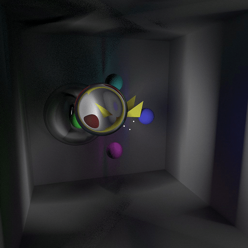
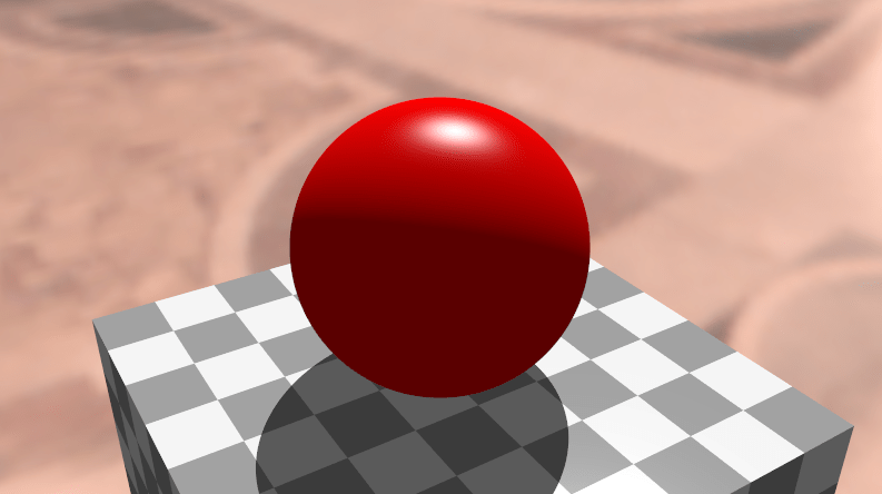
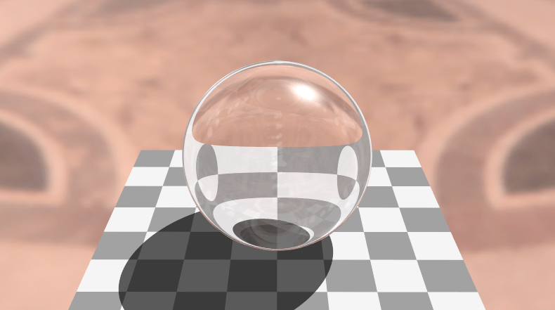
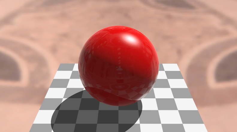
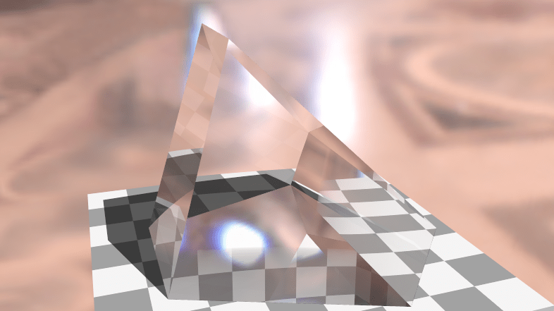
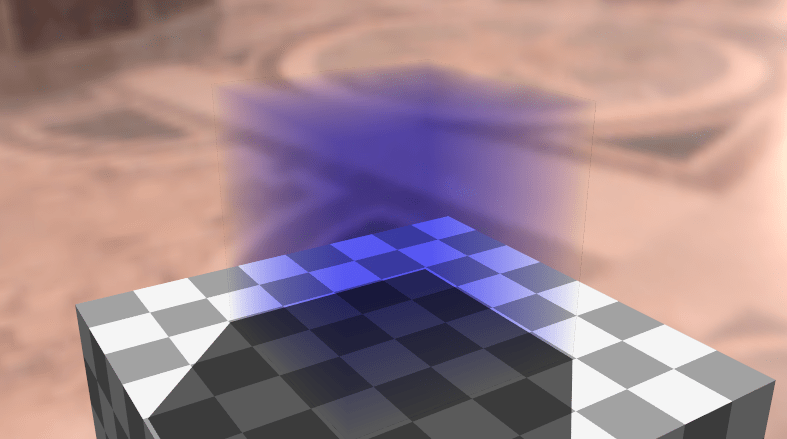
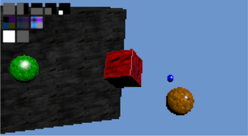
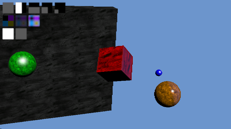
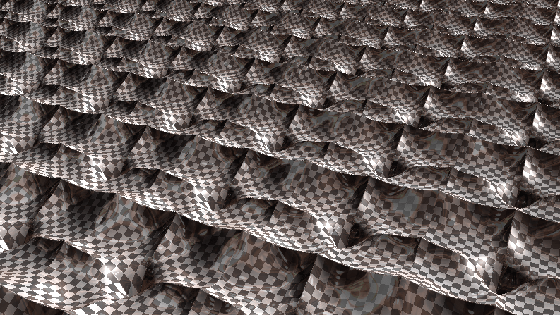
The images below were path traced using 100,000 samples per pixel, using the sample code provided in this post.

Path tracing is a specific type of ray tracing that aims to make photo realistic images by solving something called the rendering equation. Path tracing relies heavily on a method called Monte Carlo integration to get an approximate solution. In fact, it’s often called “Monte Carlo Path Tracing”, but I’ll refer to it as just “Path Tracing”.

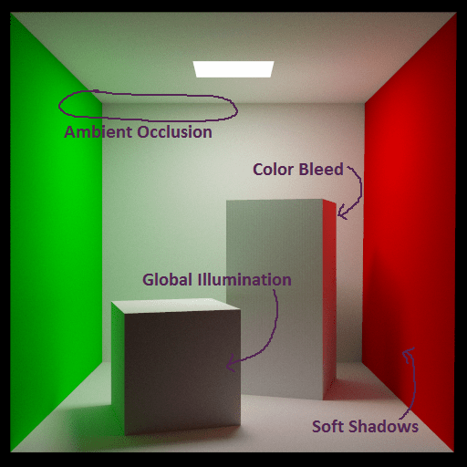
In solving the rendering equation, path tracing automatically gets many graphical “features” which are cutting edge research topics of real time graphics, such as soft shadows, global illumination, color bleeding and ambient occlusion.

Unfortunately, path tracing can take a very long time to render – like minutes, hours, or days even, depending on scene complexity, image quality desired and specific algorithms used. Despite that, learning path tracing can still be very useful for people doing real time rendering, as it can give you a “ground truth” to compare your real time approximating algorithms to, and can also help you understand the underlying physical processes involved, to help you make better real time approximations. Sometimes even, data is created offline using path tracing, and is “baked out” so that it can be a quick and simple lookup during runtime.

There is a lot of really good information out there about path tracing, walking you through the rendering equations, monte carlo integration, and the dozen or so relevant statistical topics required to do monte carlo integration.

While understanding that stuff is important if you really want to get the most out of path tracing, this series of blog posts is meant to be more informal, explaining more what to do, and less deeply about why to do it.

When and if you are looking for resources that go deeper into the why, I highly recommend starting with these!

Source Code

You can find the source code that goes along with this post here:

Github: Atrix256/RandomCode/PTBlogPost1/

You can also download a zip of the source code here:

PTBlogPost1.zip

The Rendering Equation

The rendering equation might look a bit scary at first but stay with me, it is actually a lot simpler than it looks.

L_o( \omega_o)= L_e(\omega_o)+\int_{\Omega}{f(\omega_i, \omega_o)L_i(\omega_i)(\omega_i \cdot n)\mathrm{d}\omega_i}

Here’s a simplified version:

LightOut(ViewDirection) = EmissiveLight(ViewDirection) + ReflectedLight(ViewDirection,AllDirections)

In other words, the light you see when looking at an object is made up of how much it glows in your direction (like how a lightbulb or a hot coal in a fireplace glows), and also how much light is reflected in your direction, from light that is hitting that point on the object from all other directions.

It’s pretty easy to know how much an object is glowing in a particular direction. In the sample code, I just let a surface specify how much it glows (an emissive color) and use that for the object’s glow at any point on the surface, at any viewing angle.

The rest of the equation is where it gets harder. The rest of the equation is this:

\int_{\Omega}{f(\omega_i, \omega_o)L_i(\omega_i)(\omega_i \cdot n)\mathrm{d}\omega_i}

The integral (the \int_{\Omega} at the front and the \mathrm{d}\omega_i at the back) just means that we are going to take the result of everything between those two symbols, and add them up for every point in a hemisphere, multiplying each value by the fractional size of the point’s area for the hemisphere. The hemisphere we are talking about is the positive hemisphere surrounding the normal of the surface we are looking at.

One of the reasons things get harder at this point is that there are an infinite number of points on the hemisphere.

Let’s ignore the integral for a second and talk about the rest of the equation. In other words, lets consider only one of the points on the hemisphere for now.

  • f(\omega_i, \omega_o) – This is the “Bidirectional reflectance distribution function”, otherwise known as the BRDF. It describes how much light is reflected towards the view direction, of the light coming in from the point on the hemisphere we are considering.
  • L_i(\omega_i) – This is how much light is coming in from the point on the hemisphere we are considering.
  • (\omega_i \cdot n) – This is the cosine of the angle between the point on the hemisphere we are considering and the surface normal, gotten via a dot product. What this term means is that as the light direction gets more perpendicular to the normal, light is reflected less and less. This is based on the actual behavior of light and you can read more about it here if you want to: Wikipedia: Lambert’s Cosine Law. Here is another great link about it lambertian.pdf. (Thanks for the link Jay!)

So what this means is that for a specific point on the hemisphere, we find out how much light is coming in from that direction, multiply it by how much the BRDF says light should be reflected towards the view direction from that direction, and then apply Lambert’s cosine law to make light dimmer as the light direction gets more perpendicular with the surface normal (more parallel with the surface).

Hopefully that makes enough sense.

Bringing the integral back into the mix, we have to sum up the results of that process for each of the infinite points on the hemisphere, multiplying each value by the fractional size of the point’s area for the hemisphere. When we’ve done that, we have our answer, and have our final pixel color.

This is where Monte Carlo integration comes in. Since we can’t really sum the infinite points, multiplied by their area (which is infinitely small), we are instead going to take a lot of random samples of the hemisphere and average them together. The more samples we take, the closer we get to the actual correct value. Not too hard right?

Now that we have the problem of the infinite points on the hemisphere solved, we actually have a second infinity to deal with.

The light incoming from a specific direction (a point on the hemisphere) is just the amount of light leaving a different object from that direction. So, to find out how much light is coming in from that direction, you have to find what object is in that direction, and calculate how much light is leaving that direction for that object. The problem is, the amount of light leaving that direction for that object is in fact calculated using the rendering equation, so it in turn is based on light leaving a different object and so on. It continues like this, possibly infinitely, and even possibly in loops, where light bounces between objects over and over (like putting two mirrors facing eachother). We have possibly infinite recursion!

The way this is dealt with in path tracers is to just limit the maximum amount of bounces that are considered. Higher numbers of bounces gives diminishing returns in general, so usually it’s just the first couple of bounces that really make a difference. For instance, the images at the top of this post were made using 5 bounces.

The Algorithm

Now that we know how the rendering equation works, and what we need to do to solve it, let’s write up the algorithm that we perform for each pixel on the screen.

  1. First, we calculate the camera ray for the pixel.
  2. If the camera ray doesn’t hit an object, the pixel is black.
  3. If the camera ray does hit an object, the pixel’s color is determined by how much light that object is emitting and reflecting down the camera ray.
  4. To figure out how much light that is, we choose a random direction in the hemisphere of that object’s normal and recurse.
  5. At each stage of the recursion, we return: EmittedLight + 2 * RecursiveLight * Dot(Normal, RandomHemisphereAngle) * SurfaceDiffuseColor.
  6. If we ever reach the maximum number of bounces, we return black for the RecursiveLight value.

We do the above multiple times per pixel and average the results together. The more times we do the process (the more samples we have), the closer the result gets to the correct answer.

By the way, the multiplication by 2 in step five is a byproduct of some math that comes out of integrating the BRDF. Check the links i mentioned at the top of the post for more info, or you can at least verify that I’m not making it up by seeing that wikipedia says the same thing. There is also some nice psuedo code there! (:
Wikipedia: Path Tracing: Algorithm

Calculating Camera Rays

There are many ways to calculate camera rays, but here’s the method I used.

In this post we are going to path trace using a pin hole camera. In a future post we’ll switch to using a lens to get interesting lens effects like depth of field.

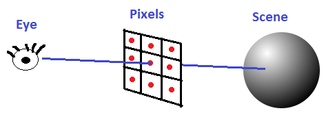
To generate rays for our pin hole camera, we’ll need an eye position, a target position that the eye is looking at, and an imaginary grid of pixels between the eye and the target.

This imaginary grid of pixels is what is going to be displayed on the screen, and may be thought of as the “near plane”. If anything gets between the eye and the near plane it won’t be visible.

To calculate a ray for a pixel, we get the direction from the eye to the pixel’s location on the grid and normalize that. That gives us the ray’s direction. The ray’s starting position is just the pixel’s location on that imaginary grid.

I’ll explain how to do this below, but keep in mind that the example code also does this process, in case reading the code is easier than reading a description of the math used.

First we need to figure out the orientation of the camera:

  1. Calculate the camera’s forward direction by normalizing (Target – Eye).
  2. To calculate the camera’s right vector, cross product the forward vector with (0,1,0).
  3. To calculate the camera’s up vector, cross product the forward vector with the right vector.

Note that the above assumes that there is no roll (z axis rotation) on the camera, and that it isn’t looking directly up.

Next we need to figure out the size of our near plane on the camera’s x and y axis. To calculate this, we have to define both a near plane distance (I use 0.1 in the sample code) as well as a horizontal and vertical field of view (I use a FOV of 40 degrees both horizontally and vertically, and make a square image, in the sample code).

You can get the size of the window on each axis then like this:

  1. WindowRight = tangent(HorizontalFOV / 2) * NearDistance
  2. WindowTop = tangent(VerticalFOV / 2) * NearDistance

Note that we divide the field of view by 2 on each axis because we are going to treat the center of the near plane as (0,0). This centers the near plane on the camera.

Next we need to figure out where our pixel’s location is in world space, when it is at pixel location (x,y):

  1. Starting at the camera’s position, move along the camera’s forward vector by whatever your near plane distance is (I use a value of 0.1). This gets us to the center of the imaginary pixel grid.
  2. Next we need to figure out what percentage on the X and Y axis our pixel is. This will tell us what percentage on the near plane it will be. We divide x by ScreenWidth and y by ScreenHeight. We then put these percentages in a [-1,1] space by multiplying the percentages by 2 and subtracting 1. We will call these values u and v, which equate to the x and y axis of the screen.
  3. Starting at the center of the pixel grid that we found, we are going to move along the camera’s right vector a distance of u and the camera’s up vector a distance of v.

We now have our pixel’s location in the world.

Lastly, this is how we calculate the ray’s position and direction:

  1. RayDir = normalize(PixelWorld – Eye)
  2. RayStart = PixelWorld

We now have a ray for our pixel and can start solving eg ray vs triangle equations to see what objects in the scene our ray intersects with.

That’s basically all there is to path tracing at a high level. Next up I want to talk about some practical details of path tracing.

Rendering Parameters, Rendering Quality and Rendering Time

A relevant quote from @CasualEffects:

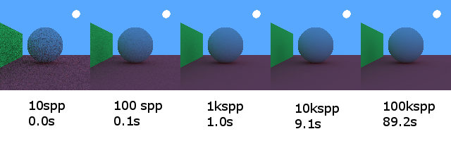
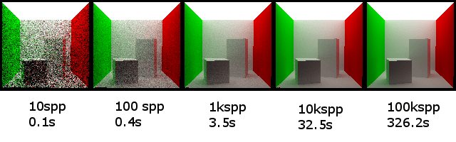
Below are a few scenes rendered at various samples per pixel (spp) and their corresponding rendering times. They are rendered at 128×128 with 5 bounces. I used 8 threads to utilize my 8 cpu cores. Exact machine specs aren’t really important here, I just want to show how sample count affects render quality and render times in a general way.


There’s a couple things worth noting.

First, render time grows roughly linearly with the number of samples per pixel. This lets you have a pretty good estimate how long a render will take then, if you know how long it took to render 1000 samples per pixel, and now you want to make a 100,000 samples per pixel image – it will take roughly 100 times as long!

Combine that with the fact that you need 4 times as many samples to half the amount of error (noise) in an image and you can start to see why monte carlo path tracing takes so long to render nice looking images.

This also applies to the size of your render. The above were rendered at 128×128. If we instead rendered them at 256×256, the render times would actually be four times as long! This is because our image would have four times as many pixels, which means we’d be taking four times as many samples (at the same number of samples per pixel) to make an image of the same quality at the higher resolution.

You can affect rendering times by adjusting the maximum number of bounces allowed in your path tracer as well, but that is not as straightforward of a relationship to rendering time. The rendering time for a given number of bounces depends on the complexity and geometry of the scene, so is very scene dependent. One thing you can count on though is that decreasing the maximum number of bounces will give you the same or faster rendering times, while increasing the maximum number of bounces will give you the same or slower rendering times.

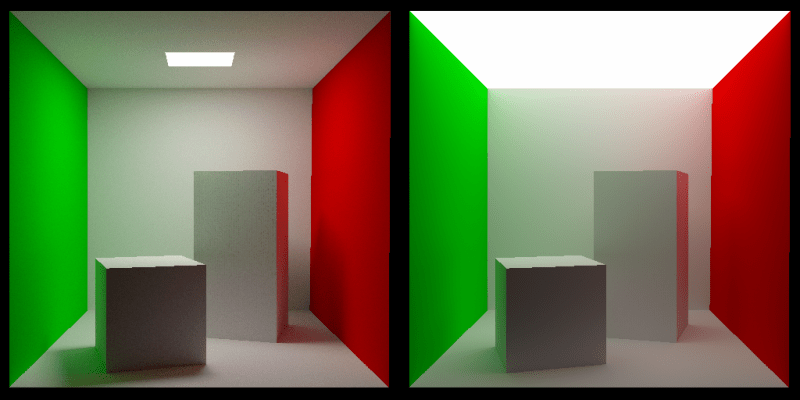
Something else that’s really important to note is that the first scene takes a lot more samples to start looking reasonable than the second scene does. This is because there is only one small light source in the first image but there is a lot of ambient light from a blue sky in the second image. What this means is that in the first scene, many rays will hit darkness, and only a few will hit light. In the second scene, many rays will hit either the small orb of light, or will hit the blue sky, but all rays will hit a light source.

The third scene also takes a lot more samples to start looking reasonable compared to the fourth scene. This is because in the third scene, there is a smaller, brighter light in the middle of the ceiling, while in the fourth scene there is a dimmer but larger light that covers the entire ceiling. Again, in the third scene, rays are less likely to hit a light source than in the fourth scene.

Why do these scenes converge at different rates?

Well it turns out that the more difference there is in the things your rays are likely to hit (this difference is called variance, and is the source of the “noisy look” in your path tracing), the longer it takes to converge (find the right answer).

This makes a bit of sense if you think of it just from the point of view of taking an average.

If you have a bunch of numbers with an average of N, but the individual numbers vary wildly from one to the next, it will take more numbers averaged together to get closer to the actual average.

If on the other hand, you have a bunch of numbers with an average of N that aren’t very different from eachother (or very different from N), it will take fewer numbers to get closer to the actual average.

Taken to the extreme, if you have a bunch of numbers with an average of N, that are all exactly the value N, it only takes one sample to get to the actual true average of N!

You can read a discussion on this here: Computer Graphics Stack Exchange: Is it expected that a naive path tracer takes many, many samples to converge?

There are lots of different ways of reducing variance of path tracing in both the sampling, as well as in the final image.

Some techniques actually just “de-noise” the final image rendered with lower sample counts. Some techniques use some extra information about each pixel to denoise the image in a smarter way (such as using a Z buffer type setup to do bilateral filtering).

Here’s such a technique that has really impressive results. Make sure and watch the video!

Nonlinearly Weighted First-order Regression for Denoising Monte Carlo Renderings

There is also a nice technique called importance sampling where instead of shooting the rays out in a uniform random way, you actually shoot your rays in directions that matter more and will get you to the actual average value faster. Importance sampling lets you get better results with fewer rays.

In the next post or two, I’ll show a very simple importance sampling technique (cosine weighted hemisphere sampling) and hope in the future to show some more sophisticated importance sampling methods.

Some Other Practical Details

Firstly, I want to mention that this is called “naive” path tracing. There are ways to get better images in less time, and algorithms that are better suited for different scenes or different graphical effects (like fog or transparent objects), but this is the most basic, and most brute force way to do path tracing. We’ll talk about some ways to improve it and get some more features in future posts.

Hitting The Wrong Objects

I wanted to mention that when you hit an object and you calculate a random direction to cast a new ray in, there’s some very real danger that the new ray you cast out will hit the same object you just hit! This is due to the fact that you are starting the ray at the collision point of the object, and the floating point math may or may not consider the new ray to hit the object at time 0 or similar.

One way to deal with this is to move the ray’s starting point a small amount down the ray direction before testing the ray against the scene. If pushed out far enough (I use a distance of 0.001) it will make sure the ray doesn’t hit the same object again. It sounds like a dodgy thing to do, because if you don’t push it out enough (how far is enough?) it will give you the wrong result, and if you push it out too far to be safe, you can miss thin objects, or can miss objects that are very close together. In practice though, this is the usual solution to the problem and works pretty well without too much fuss. Note that this is a problem in all ray tracing, not just path tracing, and this solution of moving the ray by a small epsilon is common in all forms of ray tracing I’ve come across!

Another way to deal with the problem is to give each object a unique ID and then when you cast a ray, tell it to ignore the ID of the object you just hit. This works flawlessly in practice, so long as your objects are convex – which is usually the case for ray tracing since you often use triangles, quads, spheres, boxes and similar to make your scene. However, this falls apart when you are INSIDE of a shape (like how the images at the top of this post show objects INSIDE a box), and it also falls apart when you have transparent objects, since sometimes it is appropriate for an object to be intersected again by a new ray.

I used to be a big fan of object IDs, but am slowly coming to terms with just pushing the ray out a little bit. It’s not so bad, and handles transparents and being inside an object (:

Gamma Correction

After we generate our image, we need to apply gamma correction by taking each color channel to the power of 1/2.2. A decent approximation to that is also to just take the square root of each color channel, as the final value for that color channel. You can read about why we do this here: Understanding Gamma Correction

HDR vs LDR

There is nothing in our path tracer that has any limitations on how bright something can be. We could have a bright green light that had a color value of (0, 100000, 0)! Because of this, the final pixel color may not necessarily be less than one (but it will be a positive number). Our color with be a “High Dynamic Range” color aka HDR color. You can use various tone mapping methods to turn an HDR color into an LDR color – and we will be looking at that in a future post – but for now, I am just clamping the color value between 0 and 1. It’s not the best option, but it works fine for our needs right now.

Divide by Pi?

When looking at explanations or implementations of path tracing, you’ll see that some of them divide colors by pi at various stages, and others don’t. Since proper path tracing is very much about making sure you have every little detail of your math correct, you might wonder whether you should be dividing by pi or not, and if so, where you should do that. The short version is it actually doesn’t really matter believe it or not!

Here are two great reads on the subject for a more in depth answer:
PI or not to PI in game lighting equation
Adopting a physically based shading model

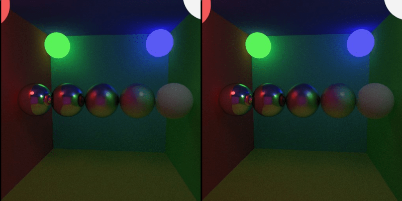
Random Point on Sphere and Bias

Correctly finding a uniformly random point on a sphere or hemisphere is actually a little bit more complicated that you might expect. If you get it wrong, you’ll introduce bias into your images which will make for some strange looking things.

Here is a good read on some ways to do it correctly:
Wolfram Math World: Sphere Point Picking

Here’s an image where the random point in sphere function was just completely wrong:

Here’s an image where the the random hemisphere function worked by picking a random point in a cube and normalizing the resulting vector (and multiplying it by -1 if it was in the wrong hemisphere). That gives too much weighting to the corners, which you can see manifests itself in the image on the left as weird “X” shaped lighting (look at the wall near the green light), instead of on the right where the lighting is circular. Apologies if it’s hard to distinguish. WordPress is converting all my images to 8BPP! :X

Primitive Types & Counts Matter

Here are some render time comparisons of the Cornell box scene rendered at 512×512, using 5 bounces and 100 samples per pixel.

There are 3 boxes which only have 5 sides – the two boxes inside don’t have a bottom, and the box containing the boxes doesn’t have a front.

I started out by making the scene with 30 triangles, since it takes 2 triangles to make a quad, and 5 quads to make a box, and there are 3 boxes.

Those 30 triangles rendered in 21.1 seconds.

I then changed it from 30 triangles to 15 quads.

It then took 6.2 seconds to render. It cut the time in half!

This is not so surprising though. If you look at the code for ray vs triangle compared to ray vs quad, you see that ray vs quad is just a ray vs triangle test were we first test the “diagonal line” of the quad, to see which of the 2 corners should be part of the ray vs triangle test. Because of this, testing a quad is just about as fast as testing a triangle. Since using quads means we have half the number of primitives, turning our triangles into quads means our rendering time is cut in half.

Lastly, i tried turning the two boxes inside into oriented boxes that have a width, height, depth, an axis of rotation and an angle of rotation around that axis. The collision test code puts the ray into the local space of the oriented box and then just does a ray vs axis aligned box test.

Doing that, i ended up with 5 quads (for the box that doesn’t have a front, it needed to stay quads, unless i did back face culling, which i didn’t want to) and two oriented boxes.

The render time for that was 5.5 seconds, so it did shave off 0.7 seconds, which is a little over 11% of the rendering time. So, it was worth while.

For such a low number of primitives, I didn’t bother with any spatial acceleration structures, but people do have quite a bit of luck on more complex scenes with bounding volume hierarchies (BVH’s).

For naive path tracing code, since the first ray hit is entirely deterministic which object it will hit (if any), we could also cache that first intersection and re-use it for each subsequent sample. That ought to make a significant difference to rendering times, but basically in the next path tracing post we’ll be removing the ability to do that, so I didn’t bother to try it and time it.

Debugging

As you are working on your path tracer, it can be useful to render an image at a low number of samples so that it’s quick to render and you can see whether things are turning out the way you want or not.

Another option is to have it show you the image as it’s rendering more and more samples per pixel, so that you can see it working.

If you make a “real time” visualizer like that, some real nice advice from Morgan McGuire (Computer graphics professor and the author of http://graphicscodex.com/) is to make a feature where if you click on a pixel, it re-renders just that pixel, and does so in a single thread so that you can step through the process of rendering that pixel to see what is going wrong.

I personally find a lot of value in visualizing per-pixel values in the image to see how values look across the pixels to be able to spot problems. You can do this by setting the emissive lighting to be based on the value you want to visualize and setting the bounce count to 1, or other similar techniques.

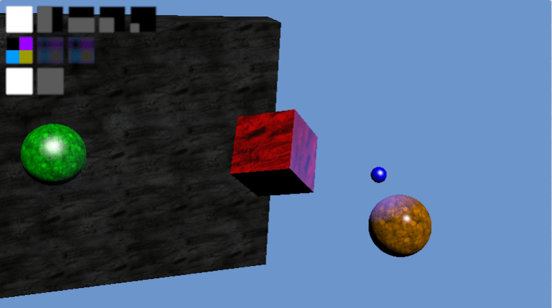
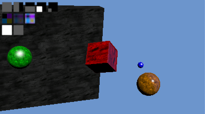
Below are two debug images I made while writing the code for this post to try and understand how some things were going wrong. The first image shows the normals of the surface that the camera rays hit (i put x,y,z of the normal into r,g,b but multiply the values by 0.5 and add 0.5 to make them be 0 to 1, instead of -1 to 1). This image let me see that the normals coming out of my ray vs oriented box test were correct.

The second image shows the number of bounces done per pixel. I divided the bounce count by the maximum number of bounces and used that as a greyscale value for the pixel. This let me see that rays were able to bounce off of oriented boxes. A previous image that I don’t have anymore showed darker sides on the boxes, which meant that the ray bouncing wasn’t working correctly.

Immensely Parallelizable: CPU, GPU, Grid Computing

At an image size of 1024×1024, that is a little over 1 million pixels.

At 1000 samples per pixel, that means a little over 1 billion samples.

Every sample of every pixel only needs one thing to do it’s work: Read only access to the scene.

Since each of those samples are able to do their work independently, if you had 1 billion cores, path tracing could use them all!

The example code is multithreaded and uses as many threads as cores you have on your CPU.

Since GPUs are meant for massively parallelizable work, they can path trace much faster than CPUs.

I haven’t done a proper apples to apples test, but evidence indicates something like a 100x speed up on the GPU vs the CPU.

You can also distribute work across a grid of computers!

One way to do path tracing in grid computing would be to have each machine do a 100 sample image, and then you could average all of those 100 sample images together to get a much higher sample image.

The downside to that is that network bandwidth and disk storage pays the cost of the full size image for each computer you have helping.

A better way to do it would probably be to make each machine do all of the samples for a small portion of the image and then you can put the tiles together at the end.

While decreasing network bandwidth and disk space usage, this also allows you to do all of the pixel averaging in floating point, as opposed to doing it in 8 bit 0-255 values like you’d get from a bmp file made on another machine.

Closing

In this post and the sample code that goes with it, we are only dealing with a purely diffuse (lambertian) surface, and emissive lighting. In future posts we’ll cover a lot more features like specular reflection (mirror type reflection), refraction (transparent objects), caustics, textures, bump mapping and more. We’ll also look at how to make better looking images with fewer samples and lots of other things too.

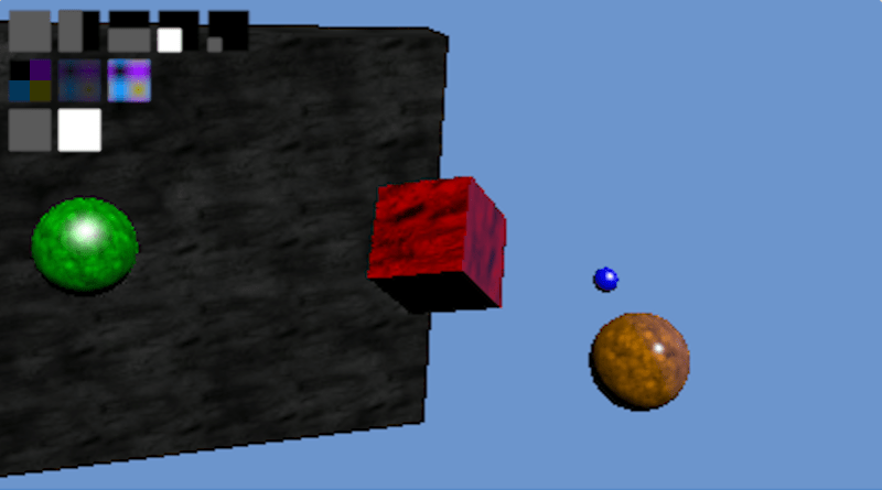
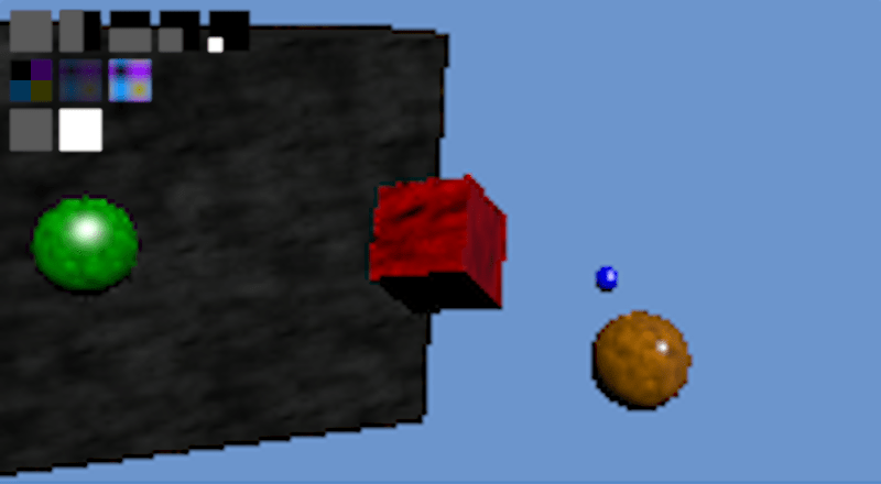
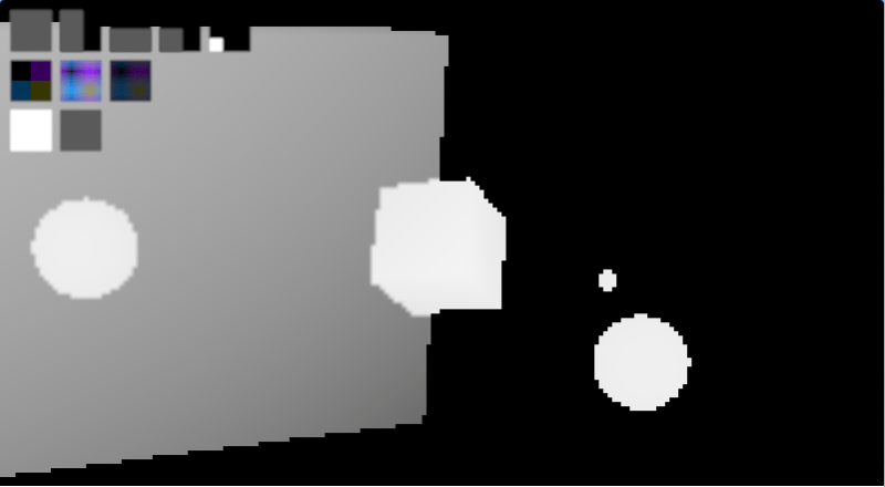
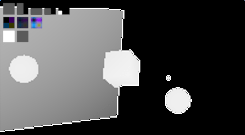
I actually have to confess that I did a bit of bait and switch. The images at the top of this post were rendered with an anti aliasing technique, as well as an importance sampling technique (cosine weighted hemisphere samples) to make the image look better faster. These things are going to be the topics of my next two path tracing posts, so be on the lookout! Here are the same scenes with the same number of samples, but with no AA, and uniform hemisphere sampling:

And the ones at the top for comparison:

While making this post I received a lot of good information from the twitter graphics community (see the people I’m following and follow them too! @Atrix256) as well as the Computer Graphics Stack Exchange.

Also, two specific individuals helped me out quite a bit:

@lh0xfb – She was also doing a lot of path tracing at the time and helped me understand where some of my stuff was going wrong, including replicating my scenes in her renderer to be able to compare and contrast with. I was sure my renderer was wrong, because it was so noisy! It turned out that while i tended to have small light sources and high contrast scenes, Lauren did a better job of having well lit scenes that converged more quickly.

@Reedbeta – He was a wealth of information for helping me understand some details about why things worked the way they did and answered a handful of graphics stack exchange questions I posted.

Thanks a bunch to you both, and to everyone else that participated in the discussions (:

G-Buffer Upsizing

The other day I had a thought:

Rendering smaller than full screen images is super helpful for performance, but upsizing an image results in pretty bad quality vs a full resolution render.

What if instead of upsizing the final rendered image, we upsized the values that were used to shade each pixel?

In other words, what if we rendered a scene from a less than full resolution g-buffer?

I was thinking that could be useful in doing ray based graphics, not having to trace or march quite so many rays, but also perhaps it could be useful for things like reflections where a user isn’t likely to notice a drop in resolution.

I’m sure I’m not the first to think of this, but I figured I’d explore it anyways and see what I could see.

I made an interactive shadertoy demo to explore this if you want to see it first hand:
Shadertoy: G-Buffer Upsizing

Result

In short, it does look better in a lot of ways because the normals, uv coordinates and similar parameters interpolate really well, but the edges of shapes are aliased really bad (jaggies).

Check out the images below to see what i mean. The first image is a full sized render. The second image is a 1/4 sized render (half x and half y resolution). The third image is a 1/16th sized render (quarter x and quarter y resolution)


For comparison, here’s a 1/4 sized and 1/16 sized render upsized using bicubic IMAGE interpolation instead of g-buffer data interpolation:


Details & More Information

Despite the aliased results at 1/16th render size, this seems like it may be a reasonable technique at larger render sizes, depending on the level of quality you need. Doing half vertical or half horizontal resolution looks very close to the full sized image for instance. The edges are a tiny bit more aliased along one direction, but otherwise things seem decent:

Since the g-buffer has only limited space, you will probably want to bit pack multiple fields together in the same color channels. When you do that, you throw out the possibility of doing hardware interpolation unfortunately, because it interpolates the resulting bit packed value, not the individual fields that you packed in.

Even when doing the interpolation yourself in the pixel shader, for the most part you can really only store information that interpolates well. For instance, you could store a diffuse R,G,B color, but you wouldn’t want to store and then interpolate a material index. This is because you might have material index 10 (say it’s blue) next to material index 0 (say it’s green), and then when you interpolate you could end up with material index 5 which may be red. You’d get red between your blue and green which is very obviously wrong.

In my demo I did have a material index per pixel, but i just used nearest neighbor for that particular value always. To help the appearance of aliasing, I also stored an RGB diffuse color that i interpolated.

I stored the uvs in the g-buffer and sampled the textures themselves in the final shader though, to make sure and get the best texture information I could. This makes textures look great at virtually any resolution and is a lot of the reason why the result looks as good as it does IMO.

The fact that normals interpolate is a good thing, except when it comes to hard edges like the edge of the cube, or at the edge of any object really. In the case of the cube edge, it smooths the edge a little bit, making a surface that catches specular lighting and so highlights itself as being incorrect (!!). In the case of the edge of regular objects, a similar thing happens because it will interpolate between the normal at the edge of the object and the background, making a halo around the object which again catches specular lighting and highlights itself as being incorrect.

I think it could be interesting or fruitful to explore using edge detection to decide when to blend or not, to help the problem with normals, or maybe even just some edge detection based anti aliasing could be nice to make the resulting images better. The depth (z buffer value) could also maybe be used to help decide when to interpolate or not, to help the problem of halos around every object.

Interestingly, bicubic interpolation actually seems to enhance the problem areas compared to bilinear. It actually seems to highlight areas of change, where you would actually want it to sort of not point out the problems hehe. I think this is due to Runge’s phenomenon. Check out the depth information below to see what i mean. The first is bilinear, the second is bicubic:


One final side benefit of this I wanted to mention, is that if you are doing ray based rendering, where finding the geometry information per pixel can be time consuming, you could actually create your g-buffer once and re-shade it with different animated texture or lighting parameters, to give you a constant time (and very quick) render of any scene of any complexity, so long as the camera wasn’t moving, and there were no geometry changes happening. This is kind of along the same lines as the very first post I made to this blog about 4 years ago, which caches geometry in screen space tiles, allowing dirty rectangles to be used (MoriRT: Pixel and Geometry Caching to Aid Real Time Raytracing).

Anyone else go down this path and have some advice, or have any ideas on other things not mentioned? (:

Next up I think I want to look at temporal interpolation of g-buffers, to see what sort of characteristics that might have. (Quick update, the naive implementation of that is basically useless as far as i can tell: G-Buffer Temporal Interpolation).

Related Stuff

On shadertoy, casty mentioned that if you have some full res information, and some less than full res information, you can actually do something called “Joint Bilateral Upsampling” to get a better result.

Give this paper a read to learn more!
Joint Bilateral Upsampling

It turns out someone has already solved this challenge with great success. They use “the MSAA trick” to get more samples at the edges. Check out ~page 38:
GPU-Driven Rendering Pipelines

Failed Shadertoy “Dust” Game – Browsers Need To Compile Shaders Off the Main Thread!

I was working on a Dust Game on shadertoy for a few weeks and got a decent amount of the way through it. Unfortunately I hit a snag.

There’s a sad fact that browsers compile WebGL shaders on the main thread. If ever WebGL blocks for too long, browsers consider WebGL hung and reports to the user that WebGL crashed.

The shaders for my game got complex enough that they were hitting the timeout while compiling, even though I wasn’t even close to being finished. So, I simplified a bit and published it unfinished, thinking that perhaps when WebGL 2.0 comes out this summer, I can revisit it.

Unfortunately, but totally understandably, different people have different machines in the wild, and some people have computers that take longer to compile shaders than my computer does, which means that plenty of people were still “crashing”. Because of this, the shadertoy people moved my shader back to draft/private until I simplified it more since crashes are no good, even if they are not realy real crashes in the normal sense. You can still see it by direct link here if you are interested: Shadertoy: Dust Sim Sandbox (Incomplete)

I’ve spent enough time on this thing so I’m going to leave it private for now, but I really think this shows a fundamental problem with WebGL.

Since the shaders compile on the main thread (apparently in many browsers if not all!), and detect a crash/hang by timing out, it means that when you write WebGL code, you really have to either keep things super simple in your shaders, or you have to be ok with having some amount of users experiencing “crashes” when the shader compiles time out on their machine.

In other words, you have to choose between innovation and stability.

That doesn’t really bode well for a platform like WebGL that basically is all about innovation! I’m sure this same problem plagues WebVR, which means that if you want to make a WebVR experience that works well on all machines, you better not do anything very complex 😛

Despite this failure, I did succeed in making a minesweeper game though, check it out here: Shadertoy: Minesweeper

Anyways, onto the next next shadertoy! I think I’m going to try to make one of those side view physics based car/motorcycle/bicycle hill climbing games.

Update!

It turns out my understanding of the shader compiling process was a bit simplified. Read the link below for the full scoop, but in the end, the problem remains, because there doesn’t seem to be any way to query the status of the async work, so you seem to have to guess and hope you have enough work to do. In the case of shadertoy, there is no geometry to load, or things of that nature, so that makes it especially difficult to deal with.

Asynchronous Shader Compilation

Thanks to @tuan_kuranes for the better information (:

Cubic Hermite Rectangles

Time for another Frankenstein post. This time we are going to combine the following:

  1. Cubic Hermite Interpolation
  2. Rectangular Bezier Patches

The end result is going to be a Cubic Hermite Rectangle Surface like the below. Note that the curve only passes through the inner four control points, and the outer ring of 12 control points are used to determine the slope.

Just like the cubic hermite curve counterpart, a cubic hermite rectangle surface is C1 continuous everywhere, which is great for use as a way of modeling geometry, as well as just for interpolation of multidimensional data. In the image below, each checkerboard square is an individual hermite rectangle.

The links section at the bottom has links to the shadertoys I made that I got the screenshots from.

Code

Here’s some C++ code that does bicubic hermite interpolation

#include <stdio.h>
#include <array>
  
typedef std::array<float, 4> TFloat4;
typedef std::array<TFloat4, 4> TFloat4x4;
  
const TFloat4x4 c_ControlPointsX =
{
    {
        { 0.7f, 0.8f, 0.9f, 0.3f },
        { 0.2f, 0.5f, 0.4f, 0.1f },
        { 0.6f, 0.3f, 0.1f, 0.4f },
        { 0.8f, 0.4f, 0.2f, 0.7f },
    }
};
  
const TFloat4x4 c_ControlPointsY =
{
    {
        { 0.2f, 0.8f, 0.5f, 0.6f },
        { 0.6f, 0.9f, 0.3f, 0.8f },
        { 0.7f, 0.1f, 0.4f, 0.9f },
        { 0.6f, 0.5f, 0.3f, 0.2f },
    }
};
  
const TFloat4x4 c_ControlPointsZ =
{
    {
        { 0.6f, 0.5f, 0.3f, 0.2f },
        { 0.7f, 0.1f, 0.9f, 0.5f },
        { 0.8f, 0.4f, 0.2f, 0.7f },
        { 0.6f, 0.3f, 0.1f, 0.4f },
    }
};
  
void WaitForEnter ()
{
    printf("Press Enter to quit");
    fflush(stdin);
    getchar();
}
  
// t is a value that goes from 0 to 1 to interpolate in a C1 continuous way across uniformly sampled data points.
// when t is 0, this will return p[1].  When t is 1, this will return p[2].
// p[0] and p[3] are used to calculate slopes at the edges.
float CubicHermite(const TFloat4& p, float t)
{
    float a = -p[0] / 2.0f + (3.0f*p[1]) / 2.0f - (3.0f*p[2]) / 2.0f + p[3] / 2.0f;
    float b = p[0] - (5.0f*p[1]) / 2.0f + 2.0f*p[2] - p[3] / 2.0f;
    float c = -p[0] / 2.0f + p[2] / 2.0f;
    float d = p[1];

    return a*t*t*t + b*t*t + c*t + d;
}
  
float BicubicHermitePatch(const TFloat4x4& p, float u, float v)
{
    TFloat4 uValues;
    uValues[0] = CubicHermite(p[0], u);
    uValues[1] = CubicHermite(p[1], u);
    uValues[2] = CubicHermite(p[2], u);
    uValues[3] = CubicHermite(p[2], u);
    return CubicHermite(uValues, v);
}
  
int main(int argc, char **argv)
{
    // how many values to display on each axis. Limited by console resolution!
    const int c_numValues = 4;
  
    printf("Cubic Hermite rectangle:n");
    for (int i = 0; i < c_numValues; ++i)
    {
        float iPercent = ((float)i) / ((float)(c_numValues - 1));
        for (int j = 0; j < c_numValues; ++j)
        {
            if (j == 0)
                printf("  ");
            float jPercent = ((float)j) / ((float)(c_numValues - 1));
            float valueX = BicubicHermitePatch(c_ControlPointsX, jPercent, iPercent);
            float valueY = BicubicHermitePatch(c_ControlPointsY, jPercent, iPercent);
            float valueZ = BicubicHermitePatch(c_ControlPointsZ, jPercent, iPercent);
            printf("(%0.2f, %0.2f, %0.2f) ", valueX, valueY, valueZ);
        }
        printf("n");
    }
    printf("n");
  
    WaitForEnter();
    return 0;
}

And here’s the output. Note that the four corners of the output correspond to the four inner most points defined in the data!

On The GPU / Links

While cubic Hermite rectangles pass through all of their control points like Lagrange surfaces do (and like Bezier rectangle’s don’t), they don’t suffer from Runge’s Phenomenon like Lagrange surfaces do.

However, just like Lagrange surfaces, Hermite surfaces don’t have the nice property that Bezier surfaces have, where the surface is guaranteed to stay inside of the convex hull defined by the control points.

Since Hermite surfaces are just cubic functions though, you could calculate the minimum and maximum value that they can reach using some calculus and come up with a bounding box by going that direction. The same thing is technically true of Lagrange surfaces as well for what it’s worth.

Check out the links below to see cubic Hermite rectangles rendered in real time in WebGL using raytracing and raymarching:
Shadertoy: Cubic Hermite Rectangle
Shadertoy: Infinite Hermite Rectangles

Lagrange Rectangles

In this post we are going to Frankenstein ideas from two other recent posts. If you haven’t seen these yet you should probably give them a read!

Ingredient 1: Lagrange interpolation
Ingredient 2: Rectangular Bezier Patches

Lagrange Surface

Lets say you have a grid of size MxN and you want to make a 3d surface for that grid.

You could use a Bezier rectangle but lets say that you really need the surface to pass through the control points. Bezier curves and surfaces only generally pass through the end / edge control points.

So what do you do? How about using Lagrange interpolation instead?

Just like how Bezier rectangles work, you interpolate on one axis, and then take those values and interpolate on the other axis.

Doing that, you get something like the below:

This comes at a price though. Whereas a Bezier curve or surface will be completely contained by it’s control points, a Lagrange rectangle isn’t always. Also, they are subject to something called Runge’s Phenomenon which basically means that the more control points you add, the more likely a surface is to get a bit “squirly”. You can see this effect when you add a lot of control points to my 1d lagrange interpolation demo as well: HTML5 1d Lagrange Interpolation.

Below is a picture of a bicubic Lagrange rectangle using the same control points the cubic Bezier rectangles used. Notice how much more extreme the peaks and valleys are! In the screenshot above, i scaled down the control points to 1/3 of what they were in the Bezier demo to make it look more reasonably well behaved.

Code

#include <stdio.h>
#include <array>
 
typedef std::array<float, 3> TFloat3;
typedef std::array<TFloat3, 3> TFloat3x3;
 
const TFloat3x3 c_ControlPointsX =
{
    {
        { 0.7f, 0.8f, 0.9f },
        { 0.2f, 0.5f, 0.4f },
        { 0.6f, 0.3f, 0.1f },
    }
};
 
const TFloat3x3 c_ControlPointsY =
{
    {
        { 0.2f, 0.8f, 0.5f },
        { 0.6f, 0.9f, 0.3f },
        { 0.7f, 0.1f, 0.4f },
    }
};
 
const TFloat3x3 c_ControlPointsZ =
{
    {
        { 0.6f, 0.5f, 0.3f },
        { 0.7f, 0.1f, 0.9f },
        { 0.8f, 0.4f, 0.2f },
    }
};
 
void WaitForEnter ()
{
    printf("Press Enter to quit");
    fflush(stdin);
    getchar();
}
 
//=======================================================================================
float QuadraticLagrange (const TFloat3& p, float t)
{
	float c_x0 = 0.0 / 2.0;
	float c_x1 = 1.0 / 2.0;
	float c_x2 = 2.0 / 2.0;

    return
        p[0] * 
        (
            (t - c_x1) / (c_x0 - c_x1) * 
            (t - c_x2) / (c_x0 - c_x2)
        ) +
        p[1] * 
        (
            (t - c_x0) / (c_x1 - c_x0) * 
            (t - c_x2) / (c_x1 - c_x2)
        ) +
        p[2] * 
        (
            (t - c_x0) / (c_x2 - c_x0) * 
            (t - c_x1) / (c_x2 - c_x1)
        );
}
 
float BiquadraticLagrangePatch(const TFloat3x3& p, float u, float v)
{
    TFloat3 uValues;
    uValues[0] = QuadraticLagrange(p[0], u);
    uValues[1] = QuadraticLagrange(p[1], u);
    uValues[2] = QuadraticLagrange(p[2], u);
    return QuadraticLagrange(uValues, v);
}
 
int main(int argc, char **argv)
{
    // how many values to display on each axis. Limited by console resolution!
    const int c_numValues = 4;
 
    printf("Lagrange rectangle:n");
    for (int i = 0; i < c_numValues; ++i)
    {
        float iPercent = ((float)i) / ((float)(c_numValues - 1));
        for (int j = 0; j < c_numValues; ++j)
        {
            if (j == 0)
                printf("  ");
            float jPercent = ((float)j) / ((float)(c_numValues - 1));
            float valueX = BiquadraticLagrangePatch(c_ControlPointsX, jPercent, iPercent);
            float valueY = BiquadraticLagrangePatch(c_ControlPointsY, jPercent, iPercent);
            float valueZ = BiquadraticLagrangePatch(c_ControlPointsZ, jPercent, iPercent);
            printf("(%0.2f, %0.2f, %0.2f) ", valueX, valueY, valueZ);
        }
        printf("n");
    }
    printf("n");
 
    WaitForEnter();
    return 0;
}

And here is the output:

Compare that to the output of the Bezier rectangles code which used the same control points:

Links

Shadertoy: Cubic Lagrange Rectangle

Note that the above uses Lagrange interpolation on a grid. The paper below talks about a way to make a Lagrange surface without using a grid:
A Simple Expression for Multivariate Lagrange Interpolation

Rectangular Bezier Patches

Rectangular Bezier Patches are one way to bring Bezier curves into the 3rd dimension as a Bezier surface. Below is a rendered image of a quadratic Bezier rectangle (degree of (2,2)) and a cubic Bezier rectangle (degree of (3,3)) taken as screenshots from a shadertoy demo I created that renders these in real time. Links at bottom of post!


Intuition

Imagine that you had a Bezier curve with some number of control points. Now, imagine that you wanted to animate those control points over time instead of having a static curve.

One way to do this would be to just have multiple sets of control points as key frames, and just linearly interpolate between the key frames over time. You’d get something that might look like the image below (lighter red = farther back in time).

That is a simple and intuitive way to animate a Bezier curve, and is probably what you thought of immediately. Interestingly though, since linear interpolation is really a degree 1 Bezier curve, this method is actually using a degree 1 Bezier curve to control each control point!

What if we tried a higher order curve to animate each control point? Well… we could have three sets of control points, so that each control point was controlled over time by a quadratic curve. We could also try having four sets of control points, so that each control point was controlled over time by a cubic curve.

We could have any number of sets of control points, to be able to animate the control points over time using any degree curve.

Now, instead of animating the curve over TIME, what if we controlled it over DISTANCE (like, say, the z-axis, or “depth”). Look at the image above and think of it like you are looking at a surface from the side. If you took a bunch of the time interpolations as slices and set them next to each other so that there were no gaps between them, you’d end up with a smooth surface. TA-DA! This is how a Rectangular Bezier Patch is made.

Note that the degree of the curve on one axis doesn’t have to match the degree of the curve on the other axis. You could have a cubic curve where each control point is controlled by a linear interpolation, or you could have a degree 5 curve where each control point is controlled by degree 7 curves. Since there are two degrees involved in a Bezier rectangle, you describe it’s order with two numbers. The first example is degree (3,1) and the second example is degree (5,7).

Higher Dimensions

While you thinking about this, I wanted to mention that you could animate a bezier rectangle over time, using bezier curves to control those control points. If you then laid that out over distance instead of time, you’d end up with a rectangular box Bezier solid. If you are having trouble visualizing that, don’t feel dumb, it’s actually four dimensional!

You can think of it like a box that has a value stored at every (x,y,z) location, and those values are controlled by Bezier formulas so are smooth and are based on control points. It’s kind of a strange concept but is useful in some situations.

Say you made a 3d hot air baloon game and wanted to model temperature of the air at differently locations to simulate thermals. One way you could do this would be to store a bunch of temperatures in a 3d grid. Another way might involve using a grid of rectangular box Bezier solids perhaps. One benefit to the Bezier solid representation is that the data points are much smoother than a grid would be, and another is that you could make the grid much less dense.

Now, let’s say that you wanted to animate the thermals over time. You could use a fifth dimensional bezier hypercube solid. Let’s move on, my brain hurts 😛

Math

The equation for a Bezier Rectangle is:

\mathbf{p}(u, v) = \sum_{i=0}^n \sum_{j=0}^m B_i^n(u) \; B_j^m(v) \; \mathbf{k}_{i,j}

\mathbf{p}(u, v) is the point on the surface that you get after you plug in the parameters. u and v are the parameters to the surface and should be within the range 0 to 1. These are the same thing as the t you see in Bezier curves, but there are two of them since there are two axes.

There are two Sigmas (summations) which mean that it’s a double for loop.

One of the for loops make i go from 0 to n and the other makes j go from 0 to m. m and n are the degree of each axis.

B_i^n(u) and B_i^n(u) are Bernstein polynomials (aka binomial expansion terms) just as you see in Bezier Curves – there is just one per axis.

Lastly comes the control points \mathbf{k}_{i,j}. The number of control on one axis are multiplied by the number of control points on the other axis.

A biquadratic Bezier patch has a degree of (2,2) and has 3 control points on one axis, and 3 control points on the other. That means that it has 9 control points total.

A bicubic Bezier patch has a degree of (3,3) with 4 control points on each axis, for a total of 16 control points.

If you had a patch of degree (7,1), it would have 8 control points on one axis and 2 control points on the other axis, and so would also have 16 control points total, but they would be laid out differently than a bicubic Bezier patch.

As far as actually calculating points on a curve, the above only calculates the value for a single axis for the final point on the curve. If you have three dimensional control points (X,Y,Z), you have to do the above math for each one to get the final result. This is the same as how it works for evaluating Bezier curves.

Code

#include 
#include 

typedef std::array TFloat3;
typedef std::array TFloat3x3;

const TFloat3x3 c_ControlPointsX =
{
    {
        { 0.7f, 0.8f, 0.9f },
        { 0.2f, 0.5f, 0.4f },
        { 0.6f, 0.3f, 0.1f },
    }
};

const TFloat3x3 c_ControlPointsY =
{
    {
        { 0.2f, 0.8f, 0.5f },
        { 0.6f, 0.9f, 0.3f },
        { 0.7f, 0.1f, 0.4f },
    }
};

const TFloat3x3 c_ControlPointsZ =
{
    {
        { 0.6f, 0.5f, 0.3f },
        { 0.7f, 0.1f, 0.9f },
        { 0.8f, 0.4f, 0.2f },
    }
};

void WaitForEnter ()
{
    printf("Press Enter to quit");
    fflush(stdin);
    getchar();
}

float QuadraticBezier (const TFloat3& p, float t)
{
    float s = 1.0f - t;
    float s2 = s * s;
    float t2 = t * t;

    return
        p[0] * s2 +
        p[1] * 2.0f * s * t +
        p[2] * t2;
}

float BiquadraticBezierPatch(const TFloat3x3& p, float u, float v)
{
    TFloat3 uValues;
    uValues[0] = QuadraticBezier(p[0], u);
    uValues[1] = QuadraticBezier(p[1], u);
    uValues[2] = QuadraticBezier(p[2], u);
    return QuadraticBezier(uValues, v);
}

int main(int argc, char **argv)
{
    // how many values to display on each axis. Limited by console resolution!
    const int c_numValues = 4;

    printf("Bezier rectangle:n");
    for (int i = 0; i < c_numValues; ++i)
    {
        float iPercent = ((float)i) / ((float)(c_numValues - 1));
        for (int j = 0; j < c_numValues; ++j)
        {
            if (j == 0)
                printf("  ");
            float jPercent = ((float)j) / ((float)(c_numValues - 1));
            float valueX = BiquadraticBezierPatch(c_ControlPointsX, jPercent, iPercent);
            float valueY = BiquadraticBezierPatch(c_ControlPointsY, jPercent, iPercent);
            float valueZ = BiquadraticBezierPatch(c_ControlPointsZ, jPercent, iPercent);
            printf("(%0.2f, %0.2f, %0.2f) ", valueX, valueY, valueZ);
        }
        printf("n");
    }
    printf("n");

    WaitForEnter();
    return 0;
}

And here is the output it gives:

Note that in the program above, I evaluate the surface points by evaluating one axis and then the other. This is basically the same as how I explained it at the top, where I’m effectively animating the control points over distance, then evaluating the curve slice of the surface at that specific distance.

You could also write it another way though, where you literally expand the mathematical formula to get just one expression to evaluate that takes all control points at once. I like the simplicity (of understanding) of the method I used, but the other method works just as well.

The Rendering

It’s easy enough to calculate values on a Bezier Rectangle, but what if you want to draw one?

One way is to tessellate it, or break it up into triangles and then render the triangles. You can think of it like trying to render a grid, where each point of the grid is moved to be where ever the Bezier rectangle function says it should be.

Raytracing against these objects in the general case is very difficult however, because it basically comes down to solving equations of very high degree.

Raymarching against these objects is also difficult unfortunately because while raymarching only needs to know “am i above the shape, or underneath it?”, knowing what u,v to plug into the equation to get the height most relevant to a random point in space is also very difficult. Not as difficult as the raytracing equations, but probably just as much out of reach.

But never fear, as always, you can cheat!

If you read my post about one dimensional (explicit) Bezier curves (One Dimensional Bezier Curves), you may remember that math gets easier if you use one dimensional control points. The same is actually true with Bezier rectangles!

For the ray marching case, you can march a point through space, and plug the x,z coordinate of the point into the Bezier rectangle function as u,v values and the number that comes out you can treat as a y coordinate.

Now, ray marching a Bezier rectangle is the same as ray marching any old height map (check links section for more info on that).

What I did in my demos, is since i knew that the curve was constrained to 0-1 on the x and z axis, and the y axis min and max was the control point min and maxes, I did a raytrace of that bounding box to get a minimum and maximum distance that the ray was inside that box. From there, I did raymarching from that min time to the max time along the ray, considering the ray as hitting the surface whenever the distance from the ray to the surface on the y axis (rayPos.y – bezierRectangle.y) changed sign.

After I had a hit, I got the height of the curve slightly offset on the x axis, then slightly offset on the z axis to get a triangle that I could calculate a surface normal from, to do lighting and shading with.

There is room for improvement in the ray marching though. I evenly divide the space through the box by a specific amount to control the size of the steps. A better way to do this I think would be to get the gradient of the function and use that to get a distance estimate (check links section below for more information). I could use that value to control the distance the ray marches at each step, and should be able to march through the box much quicker.

Also, as the link on terrain marching explains, you can usually take farther steps when the ray is farther from the camera, because the eye notices less detail. I removed that since the Bezier rectangles are pretty close to the camera, but it probably still would be helpful. Also, it would DEFINITELY be helpful in the case of the “Infinite Bezier Rectangles” scene.

I am pretty sure you could directly raytrace an explicit Bezier rectangle (one who has one dimensional control points) – at least for low degrees. I personally don’t know how you would do that, but I think it might boil down to solving a 4th degree function or something else “reasonable” based on a similar question I had about Bezier triangles on the mathematics stack exchange site (link below).

Another Way To Render

There is another way to render Bezier surfaces using ray based methods that I didn’t use but want to mention.

A property of Bezier curves and surfaces is that they are guaranteed to be completely contained by the convex hull created by their control points.

Another property of Bezier curves and surfaces is that you can use the De Casteljeau algorithm to cut them up. For instance you could cut a Bezier curve into two different Bezier curves, and the same holds for Bezier surfaces.

Using these two properties, there is an interesting way to be able to tell if a ray intersects a bezier curve or not, which is:

  1. If the line misses the convex hull, return a miss
  2. If the convex hull is smaller than a pixel, return a hit
  3. Otherwise, cut the Bezier object into a couple smaller Bezier objects
  4. Recurse for each smaller Bezier object

Yes, believe it or not, that is a real technique! It’s called Bezier Clipping and there is a research paper in the links section below that talks about some of the details of using that rendering technique.

Links

Lastly, I wanted to mention that the above is completely about Bezier rectangles, but there is no reason you couldn’t extend these rectangles to use rational Bezier functions, or be based on B-splines or NURBS, or even go a different direction and make hermite surfaces or catmull-rom surfaces, or even make surfaces that used exotic basis functions of your own crafting based on trigonometric functions or whatever else!

Here are the shadertoy demos I made:
Shadertoy: Cubic Bezier Rectangle
Shadertoy: Quadratic Bezier Rectangle
Shadertoy: Infinite Bezier Rectangles

And some other links about this stuff:
IQ – terrain raymarching
IQ – distance estimation (using function gradients)
Math Stack Exchange – Ray intersection with explicit (1 axis) Bezier triangle?
Math Stack Exchange – Intersect Ray (Line) vs Quadratic Bezier Triangle
Bézier Surfaces: de Casteljau’s Algorithm
Ray Tracing Triangular Bézier Patches (including Bezier clipping)
Wikipedia: Bezier Surface
Wikipedia: Bezier Triangle