Fast Voronoi Diagrams and Distance Field Textures on the GPU With the Jump Flooding Algorithm

The image below is called a Voronoi diagram. The circles show you the location of the seeds and the color of each pixel represents the closest seed to that pixel. The value of this diagram is that at any point on the image, you can know which seed (point) is the closest to that pixel. It’s basically a pre-computed “closest object” map, which you can imagine some uses for I bet.

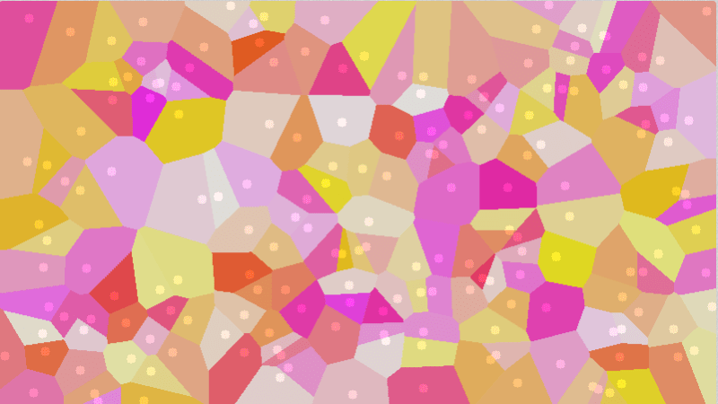
Voronoi diagrams aren’t limited to just points as seeds though, you can use any shape you want.

One way Voronoi diagrams can be useful is for path finding because they are dual to (the equivelant of) Delauny triangulation (More info at How to Use Voronoi Diagrams to Control AI).

Another way they can be useful is in generating procedural content, like in these shadertoys:
Shadertoy: Voronoi – rocks
Shadertoy: Voronoi noises

Another really cool usage case of Voronoi diagrams is in creating what is called the “Distance Transform”. The distance transform calculates and stores the distance from each pixel to the closest seed, whichever one that may be. Doing that, you may get an image like this (note that the distance is clamped at a maximum and mapped to the 0 to 1 range to make this image).

That is what is called a distance texture and can be used for a very cool technique where you have texture based images that can be zoomed into / enlarged quite a ways before breaking down and looking bad. The mustache in the image below was made with a 32×16 single channel 8bpp image for instance! (ignore the white fog, this was a screenshot from inside a project I was working on)

Distance field textures are the next best thing to vector graphics (great for scalable fonts in games, as well as decals!) and you can read about it here: blog.demofox.org: Distance Field Textures

Now that you know what Voronoi diagrams and distance transforms are used for, let’s talk about one way to generate them.

Jump Flooding Algorithm (JFA)

When you want to generate either a Voronoi diagram or a distance transform, there are algorithms which can get you the exact answer, and then there are algorithms which can get you an approximate answer and generally run a lot faster than the exact version.

The jump flooding algorithm is an algorithm to get you an approximate answer, but seems to have very little error in practice. It also runs very quickly on the GPU. It runs in constant time based on the number of seeds, because it’s execution time is based on the size of the output texture – and is based on that logarithmically.

Just a real quick note before going into JFA. If all else fails, you could use brute force to calculate both Voronoi diagrams as well as distance transforms. You would just loop through each pixel, and then for each pixel, you would loop through each seed, calculate the distance from the pixel to the seed, and just store the information for whatever seed was closest. Yes, you even do this for seed pixels. The result will be a distance of 0 to the seed 😛

Back to JFA, JFA is pretty simple to program, but understanding why it works may take a little bit of thinking.

Firstly you need to prepare the N x N texture that you want to run JFA on. It doesn’t need to be a square image but let’s make it square for the explanation. Initialize the texture with some sentinel value that means “No Data” such as (0.0, 0.0, 0.0, 0.0). You then put your seed data in. Each pixel that is a seed pixel needs to encode it’s coordinate inside of the pixel. For instance you may store the fragment coordinate bitpacked into the color channels if you have 32 bit pixels (x coordinate in r,g and y coordinate in b,a). Your texture is now initialized and ready for JFA!

JFA consists of taking log2(N) steps where each step is a full screen pixel shader pass.

In the pixel shader, you read samples from the texture in a 3×3 pattern where the middle pixel is the current fragment. The offset between each sample on each axis is 2^(log2(N) – passIndex – 1), where passIndex starts at zero.

That might be a bit hard to read so let’s work through an example.

Let’s say that you have an 8×8 texture (again, it doesn’t need to be square, or even power of 2 dimensions, but it makes it easier to explain), that has a 16 bit float per RGBA color channel. You fill the texture with (0.0, 0.0, 0.0, 0.0) meaning there is no data. Let’s say that you then fill in a few seed pixels, where the R,G channels contain the fragment coordinate of that pixel. Now it’s time to do JFA steps.

The first JFA step will be that for each pixel you read that pixel, as well as the rest of a 3×3 grid with offset 4. In total you’d read the offsets:
(-4.0, -4.0), (0.0, -4.0), (4.0, -4.0),
(-4.0, 0.0), (0.0, 0.0), (4.0, 0.0),
(-4.0, 4.0), (0.0, 4.0), (4.0, 4.0)

For each texture read you did, you calculate the distance from the seed it lists inside it (if the seed exists aka, the coordinate is not 0,0), and store the location of the closest seed int the output pixel (like, store the x,y of the seed in the r,g components of the pixel).

You then do another JFA step with offset 2, and then another JFA step with offset 1.

JFA is now done and your image will store the Voronoi diagram, that’s all! If you look at the raw texture it won’t look like anything though, so to view the Voronoi diagram, you need to make a pixel shader where it reads in the pixel value, deocdes it to get the x,y of the closest seed, and then uses that x,y somehow to generate a color (use it as a seed for a prng for instance). That color is what you would output in the pixel shader, to view the colorful Voronoi diagram.

To convert the Voronoi diagram to a distance transform, you’d do another full screen shader pass where for each pixel you’d calculate the distance from that pixel to the seed that it stores (the closest seed location) and write the distance as output. If you have a normalized texture format, you’re going to have to divide it by some constant and clamp it between 0 and 1, instead of storing the raw distance value. You now have a distance texture!

More Resources

I originally came across this algorithm on shadertoy: Shadertoy: Jump Flooding. That shadertoy was made by @paniq who is working on some pretty interesting stuff, that you can check out both on shadertoy and twitter.

The technique itself comes from this paper, which is a good read: Jump Flooding in GPU with Applications to Voronoi Diagram and Distance Transform

Extensions

While JFA as explained is a 2D algorithm, it could be used on volume textures, or higher dimensions as well. Higher dimensions mean more texture reads, but it will still work. You could render volume textures with raymarching, using the distance information as a hint for how far you could march the ray each step.

Also, I’ve played around with doing 5 reads instead of 9, doing a plus sign read instead of a 3×3 grid. In my tests it worked just as well as regular JFA, but I’m sure in more complex situations there are probably at least minor differences. Check the links section for a shadertoy implementation of this. I also tried doing a complete x axis JFA followed by a y axis JFA. That turned out to have a LOT of errors.

You can also weight the seeds of the Voronoi diagram. When you are calculating the distance from a pixel to a seed point, you use the seed weight to multiply and/or add to the distance calculated. You can imagine that perhaps not all seeds are created equal (maybe some AI should avoid something more than something else), so weighting can be used to achieve this.

Shadertoys

Here are some shadertoys I made to experiment with different aspects of this stuff. You can go check them out to see working examples of JFA in action with accompanying glsl source code.

Jump Flood Algorithm: Points – Point Seeds
Jump Flood Algorithm: Shapes – Shape Seeds
Jump Flood Algorithm: Weight Pts – Multiplicative Weighting
Jump Flood Algorithm: Add Wt Pts – Additive Weighting
Separable Axis JFA Testing – Does 5 reads instead of 9, also shows how separating axis completely fails.

Here is a really interesting shadertoy that shows a way of modifying a Vornoi diagram on the fly: Shadertoy: zoomable, stored voronoi cells

GPU Texture Sampler Bezier Curve Evaluation

Below is a paper I submitted to jcgt.org that unfortunately did not get accepted. Maybe next time!

The main idea of this paper is that bilinear interpolation can be equivalent to the De Casteljau algorithm, which means that if you set up a texture in a specific way, and sample from it at specific texture coordinates, that it will in fact give you Bezier curve points as output! It scales up for higher dimensional textures, as well as higher order curves.

The image below shows this in action for a cubic Bezier curve (3 control points) being stored and recalled from a 2×2 texture (there is actually a curve stored in each color channel).

This image is from an extension linked to lower down which applies the technique to surfaces and volumes:

The primary feedback from the reviewers and editor was that:

  • It was an interesting technique and they thought it was a paper worth reading.
  • The usage case was fairly limited though – basically only when your are compute bound in your shader program, and have some curve calculations to offload to the texture sampler. Or if you are already using a lookup texture and would benefit from fewer instructions and smaller lookup textures.
  • It could have been shorter due to the writing being shorter, but also it could have been less thorough. For instance, it didn’t need to show equivalence to both the De Casteljau’s algorithm as well as Bernstein polynomials, since it’s already known that those are equivalent.
  • They wanted some more performance details

I agree with the feedback, and don’t feel like taking the time to change and resubmit or submit else where, so I’m sharing it here on my blog. I hope you enjoy it and find it interesting (:

Here is the paper:
GPUBezier2016.pdf

Here is the supplemental materials (opengl and webgl source code):
SupplementalMaterials.zip

Here is the webgl demo from the supplemental materials, hosted on my site:
GPU Efficient Texture Based Bezier Curve Evaluation

Here are some working shadertoy demos of the technique:
Shadertoy: Mystery Curves – Quadratic
Shadertoy: Mystery Curves – Cubic
Shadertoy: Mystery Curves – Quartic
Shadertoy: Mystery Curves – Quintic

Extensions

Continuations of this work:

Failed Experiments

Continuations that didn’t work out:

What are your thoughts? Is this cool? Is it lame? Got some ideas to improve it? Leave a comment! (:

G-Buffer Upsizing

The other day I had a thought:

Rendering smaller than full screen images is super helpful for performance, but upsizing an image results in pretty bad quality vs a full resolution render.

What if instead of upsizing the final rendered image, we upsized the values that were used to shade each pixel?

In other words, what if we rendered a scene from a less than full resolution g-buffer?

I was thinking that could be useful in doing ray based graphics, not having to trace or march quite so many rays, but also perhaps it could be useful for things like reflections where a user isn’t likely to notice a drop in resolution.

I’m sure I’m not the first to think of this, but I figured I’d explore it anyways and see what I could see.

I made an interactive shadertoy demo to explore this if you want to see it first hand:
Shadertoy: G-Buffer Upsizing

Result

In short, it does look better in a lot of ways because the normals, uv coordinates and similar parameters interpolate really well, but the edges of shapes are aliased really bad (jaggies).

Check out the images below to see what i mean. The first image is a full sized render. The second image is a 1/4 sized render (half x and half y resolution). The third image is a 1/16th sized render (quarter x and quarter y resolution)


For comparison, here’s a 1/4 sized and 1/16 sized render upsized using bicubic IMAGE interpolation instead of g-buffer data interpolation:


Details & More Information

Despite the aliased results at 1/16th render size, this seems like it may be a reasonable technique at larger render sizes, depending on the level of quality you need. Doing half vertical or half horizontal resolution looks very close to the full sized image for instance. The edges are a tiny bit more aliased along one direction, but otherwise things seem decent:

Since the g-buffer has only limited space, you will probably want to bit pack multiple fields together in the same color channels. When you do that, you throw out the possibility of doing hardware interpolation unfortunately, because it interpolates the resulting bit packed value, not the individual fields that you packed in.

Even when doing the interpolation yourself in the pixel shader, for the most part you can really only store information that interpolates well. For instance, you could store a diffuse R,G,B color, but you wouldn’t want to store and then interpolate a material index. This is because you might have material index 10 (say it’s blue) next to material index 0 (say it’s green), and then when you interpolate you could end up with material index 5 which may be red. You’d get red between your blue and green which is very obviously wrong.

In my demo I did have a material index per pixel, but i just used nearest neighbor for that particular value always. To help the appearance of aliasing, I also stored an RGB diffuse color that i interpolated.

I stored the uvs in the g-buffer and sampled the textures themselves in the final shader though, to make sure and get the best texture information I could. This makes textures look great at virtually any resolution and is a lot of the reason why the result looks as good as it does IMO.

The fact that normals interpolate is a good thing, except when it comes to hard edges like the edge of the cube, or at the edge of any object really. In the case of the cube edge, it smooths the edge a little bit, making a surface that catches specular lighting and so highlights itself as being incorrect (!!). In the case of the edge of regular objects, a similar thing happens because it will interpolate between the normal at the edge of the object and the background, making a halo around the object which again catches specular lighting and highlights itself as being incorrect.

I think it could be interesting or fruitful to explore using edge detection to decide when to blend or not, to help the problem with normals, or maybe even just some edge detection based anti aliasing could be nice to make the resulting images better. The depth (z buffer value) could also maybe be used to help decide when to interpolate or not, to help the problem of halos around every object.

Interestingly, bicubic interpolation actually seems to enhance the problem areas compared to bilinear. It actually seems to highlight areas of change, where you would actually want it to sort of not point out the problems hehe. I think this is due to Runge’s phenomenon. Check out the depth information below to see what i mean. The first is bilinear, the second is bicubic:


One final side benefit of this I wanted to mention, is that if you are doing ray based rendering, where finding the geometry information per pixel can be time consuming, you could actually create your g-buffer once and re-shade it with different animated texture or lighting parameters, to give you a constant time (and very quick) render of any scene of any complexity, so long as the camera wasn’t moving, and there were no geometry changes happening. This is kind of along the same lines as the very first post I made to this blog about 4 years ago, which caches geometry in screen space tiles, allowing dirty rectangles to be used (MoriRT: Pixel and Geometry Caching to Aid Real Time Raytracing).

Anyone else go down this path and have some advice, or have any ideas on other things not mentioned? (:

Next up I think I want to look at temporal interpolation of g-buffers, to see what sort of characteristics that might have. (Quick update, the naive implementation of that is basically useless as far as i can tell: G-Buffer Temporal Interpolation).

Related Stuff

On shadertoy, casty mentioned that if you have some full res information, and some less than full res information, you can actually do something called “Joint Bilateral Upsampling” to get a better result.

Give this paper a read to learn more!
Joint Bilateral Upsampling

It turns out someone has already solved this challenge with great success. They use “the MSAA trick” to get more samples at the edges. Check out ~page 38:
GPU-Driven Rendering Pipelines

Normalized Vector Interpolation TL;DR

My blog posts often serve as “external memory”, allowing me to go back and remember how specific things work months or years after I spent the time to learn about them.

So far it’s worked amazingly well! Instead of having a hazy memory of “oh um… i did bicubic interpolation once, how does that work again?” I can go back to my blog post, find the details with an explanation and simple working code, and can very rapidly come back up to speed. I seriously recommend keeping a blog if you are a programmer or similar. Plus, you know you really understand something when you can explain it to someone else, so it helps you learn to a deeper level than you would otherwise.

Anyways, this is going to be a very brief post on vector interpolation that I want to commit to my “external memory” for the future.

This is an answer to the question… “How do I interpolate between two normalized vectors?” or “How do i bilinearly or bicubically interpolate between normalized vectors?”

As an answer I found the three most common ways to do vector interpolation:

  • Slerp – short for “spherical interpolation”, this is the most correct way, but is also the costliest. In practice you likely do not need the precision.
  • lerp – short for “linear interpolation”, you just do a regular linear interpolation between the vectors and use that as a result.
  • nlerp – short for “normalized linear interpolation” you just normalize the result of a lerp. Useful if you need your interpolated vector to be a normalized vector.

In practice, lerp/nlerp are pretty good at getting a pretty close interpolated direction so long as the angle they are interpolating between is sufficiently small (say, 90 degrees), and nlerp is of course good at keeping the right length, if you need a normalized vector. If you want to preserve the length while interpolating between non normalized vectors, you could always interpolate the length and direction separately.

Here is an example of the three interpolations on a large angle. Dark grey = start vector, light grey = end vector. Green = slerp, blue = lerp, orange = nlerp.

Here is an example of a medium sized angle (~90 degrees) interpolating the same time t between the angles.

Lastly, here’s a smaller angle (~35 degrees). You can see that the results of lerp / nlerp are more accurate as the angle between the interpolated vectors gets smaller.

If you do lerp or nlerp, you can definitely do both bilinear as well as bicubic interpolation since they are just regularly interpolated values (and then optionally normalized)

Using slerp, you can do bilinear interpolation, but I’m not sure how bicubic would translate.

I miss something important? Leave a comment and let me know!

Code

Here’s some glsl code for slerp, lerp and nlerp. This code is for vec2’s specifically but the same code works for vectors of any dimension.

//============================================================
// adapted from source at:
// https://keithmaggio.wordpress.com/2011/02/15/math-magician-lerp-slerp-and-nlerp/
vec2 slerp(vec2 start, vec2 end, float percent)
{
     // Dot product - the cosine of the angle between 2 vectors.
     float dot = dot(start, end);     
     // Clamp it to be in the range of Acos()
     // This may be unnecessary, but floating point
     // precision can be a fickle mistress.
     dot = clamp(dot, -1.0, 1.0);
     // Acos(dot) returns the angle between start and end,
     // And multiplying that by percent returns the angle between
     // start and the final result.
     float theta = acos(dot)*percent;
     vec2 RelativeVec = normalize(end - start*dot); // Orthonormal basis
     // The final result.
     return ((start*cos(theta)) + (RelativeVec*sin(theta)));
}

vec2 lerp(vec2 start, vec2 end, float percent)
{
     return mix(start,end,percent);    
}

vec2 nlerp(vec2 start, vec2 end, float percent)
{
     return normalize(mix(start,end,percent));    
}

Links

An interactive shadertoy demo I made, that is also where the above images came from:
Shadertoy: Vector Interpolation

Further discussion on this topic may be present here:
Computer Graphics Stack Exchange: Interpolating vectors on a grid

Good reads that go deeper:
Math Magician – Lerp, Slerp, and Nlerp
Understanding Slerp, Then Not Using It

How and Why Cleaning Up Code or Processes Gives Multiplicative Benefits

The engineering manager of my team Paul Haban (@XpresoAdct) mentioned to me once in passing that when you fix a problem, you often get multiplicative returns beyond the initial problem you intended to fix.

This is an idea from Kanban, and while it was in my best interest to believe this to be true, since it allowed to refactor personally painful inherited systems and code, it felt like a sort of mysterious voodoo and I wasn’t really a believer.

I recently experienced it first hand though. I refactored something and the benefits started multiplying. People from distant sub teams came out of the woodwork very excited to hear about my changes. Of course, this happens from time to time, and it’s a lucky break to get benefits beyond what you were planning, but looking at it in hindsight, there are some really good reasons why this happened.

This applies to source code, processes, etc, but for simpler language, we’ll focus on this being about code.

What is Bad Code?

Firstly, engineering is often about trade offs. You might see that solving a problem one way gives you certain benefits, while solving a problem a different way gives you other benefits. You weigh those things, talk to those affected to get their opinions in case you are missing information, and then you make the best decision you can with the information you have.

Sometimes you make a decision based on the current state of things, but then the situation changes, and the choices you make turn out to be bad choices for the new direction that things have taken. Now your code has turned bad.

Also of course, people sometimes people just make bad choices. We are human, we are learning, it’s how it goes. Sometimes people just make bad code to begin with.

A deeper chat of this sort of thing can be found here: No Bad Code, Creeping Normality and Social Structure Code Organization

But ultimately, here is what makes code “bad”: If it works less than ideally for someone or some thing that has to interact with it, it is on the spectrum of “bad code”, ranging from terrible code, to code that could be cleaned up, but doesn’t really matter enough to fix.

It also may be that code is bad for one set of interactions, while it is perfectly ideal for another set of interactions. This is the result of the trade offs weighed when solving the problem. That may just be a fact of life that you either can not really do anything about, or that in practical terms, you cannot do anything about due to cost versus reward analysis or whatever else.

Lastly, like in my case, you may have inherited some bad code from someone else. In this case, it could just be that you have different goals, or that you prefer a different trade off (pain flavor if you will) than the previous maintainer.

How Does Bad Code Affect Others

By definition, bad code is code that is less than ideal for a person, or code that has to interact with it.

That means that when they interact with the code two things happen:

  1. There are work arounds that have to be done to be able to get what is needed from the system.
  2. There may be perfectly reasonable things that interactions with the system may want to do that are not possible, or not practically possible with real world constraints.

The more central this bad code is, and the more people that interact with it, the more that there is both workarounds, and desired functionality that can’t be realized.

Refactoring

If you can legitimately refactor some code such that the result is decided to be better than where things are at now – say, there is less pain overall, or perhaps the pain is more concentrated on a group that nobody likes (hehe) – making that happen will make the code less bad.

Again, bad code is a spectrum, so it’s likely you’ll hit situations where the code will never be perfectly good code, but making it less bad is a good thing.

When you make code less bad, however you measure that, it means that the workarounds that needed to go up can start being taken down (simpler code, less maintenance, fewer things that can go wrong), and also, you open up the doorway for the improved functionality that was not previously practical.

Another way to think of it is that the optimist will say that fixing things gives multiplicative benefits. The cynic (realist?) on the other hand says that the less than ideal code has already incurred both a one time cost to the people that have interfaced with it, as well as a continual maintenance cost that is incurred by it existing, and that those costs are or were avoidable.

To me, this explains in a very down to earth way how the “voodoo” of multiplicative benefits actually comes about. It also shows a bit of how continual minor improvement really does add up (the main idea of Kanban), even when not taking into account things like the compound interest model (ie, saving you effort now allows you to save future effort sooner).

Go clean up some code, or fix a broken process. You will likely be surprised at how much benefit you get out of it!

I miss anything or you have a differing view? Let me know!

Failed Shadertoy “Dust” Game – Browsers Need To Compile Shaders Off the Main Thread!

I was working on a Dust Game on shadertoy for a few weeks and got a decent amount of the way through it. Unfortunately I hit a snag.

There’s a sad fact that browsers compile WebGL shaders on the main thread. If ever WebGL blocks for too long, browsers consider WebGL hung and reports to the user that WebGL crashed.

The shaders for my game got complex enough that they were hitting the timeout while compiling, even though I wasn’t even close to being finished. So, I simplified a bit and published it unfinished, thinking that perhaps when WebGL 2.0 comes out this summer, I can revisit it.

Unfortunately, but totally understandably, different people have different machines in the wild, and some people have computers that take longer to compile shaders than my computer does, which means that plenty of people were still “crashing”. Because of this, the shadertoy people moved my shader back to draft/private until I simplified it more since crashes are no good, even if they are not realy real crashes in the normal sense. You can still see it by direct link here if you are interested: Shadertoy: Dust Sim Sandbox (Incomplete)

I’ve spent enough time on this thing so I’m going to leave it private for now, but I really think this shows a fundamental problem with WebGL.

Since the shaders compile on the main thread (apparently in many browsers if not all!), and detect a crash/hang by timing out, it means that when you write WebGL code, you really have to either keep things super simple in your shaders, or you have to be ok with having some amount of users experiencing “crashes” when the shader compiles time out on their machine.

In other words, you have to choose between innovation and stability.

That doesn’t really bode well for a platform like WebGL that basically is all about innovation! I’m sure this same problem plagues WebVR, which means that if you want to make a WebVR experience that works well on all machines, you better not do anything very complex 😛

Despite this failure, I did succeed in making a minesweeper game though, check it out here: Shadertoy: Minesweeper

Anyways, onto the next next shadertoy! I think I’m going to try to make one of those side view physics based car/motorcycle/bicycle hill climbing games.

Update!

It turns out my understanding of the shader compiling process was a bit simplified. Read the link below for the full scoop, but in the end, the problem remains, because there doesn’t seem to be any way to query the status of the async work, so you seem to have to guess and hope you have enough work to do. In the case of shadertoy, there is no geometry to load, or things of that nature, so that makes it especially difficult to deal with.

Asynchronous Shader Compilation

Thanks to @tuan_kuranes for the better information (: