My Old Master: How to Correct as a Mentor or a Teacher

Preface: I studied martial arts for a little over a decade (shaolin kempo at USSD) and learned a lot while I was there. Our teacher was a great guy who genuinely cared about his students, and in particular, taught my friends and I some really interesting things when we became instructors. I’d like to share some of that information with you in the “My Old Master” posts category. As cliched as it is, many things he taught us apply to all aspects of life, not just martial arts and I’d like other people to benefit from them.

My old master used to say…

“Praise, Correct, Praise. Even if you have to make something up, you need to say something positive.”

Let’s say that I’m teaching you how to punch and you aren’t quite doing it right.

Here are two things I might say to try and correct it:

  1. “Keep your wrist straight when you are punching so you don’t hurt your hand” or…
  2. “I really love how you are keeping your left hand up while you punch with your right. It’s doing a great job of protecting your head against your opponent hitting you back. Now try keeping your wrist straight when you punch so that you don’t hurt your hand.” Then I watch you try again and I say “Great, just like that, keep it up!”

Think about how those two responses make you feel for a second.

The first one likely makes you feel like you are messing up and need to fix it (a negative thing), while the second makes you feel like you were doing well and are now are doing even better.

What’s the difference? Well, like the opening quote says, I praised, corrected, and then praised. First I found something you were doing well, complimented you on it, gave a suggestion for improvement, and then praised you on doing (or attempting!) the correction.

This can be a great way to give people feedback, in a way that makes them feel better about themselves, and feel better about the feedback you are giving them. Instead of being a negative thing, it becomes a positive thing.

Pretty simple stuff, and if you practice this technique it starts to become second nature.

The quote says that if you can’t find anything positive to say, you should make it up. It shouldn’t be your first choice to make something up, because the more genuine you are about the praise, the better it will be. However, if you really can’t find anything nice to say, yes, you should make something up.

A person’s ego and self worth is a measurable quantity that is increased with praise and decreased with corrections or negative feedback (aka “you suck!”). When this tank of self worth gets too low, your student or mentee will feel worthless, get frustrated and/or start to get resentful at you.

This technique is useful because it allows you to give a correction while minimizing hit to the person’s self worth. In the end allows you to give MORE correction and help them more in the long run, just by phrasing your corrections differently. Another term for this is “complement sandwich” which you may have heard of before.

Another thing to be mindful of however is that you can only give so much feedback at any one time. The ego/self worth tank needs to refill after it’s diminished, and frankly, the person needs to absorb and internalize what you’ve taught them before they are ready for more.

Our teacher would say “it’s better having a mediocre black belt, than having a stellar white belt who quits out of frustration” and that’s very true. It’s better for them since a mediocre black belt is FAR SUPERIOR to a stellar white belt and much better able to protect themselves and their loved ones, but also better for the organization, since we are often teaching or mentoring in a “for profit” situation where the person we are trying to help is either a customer or a co-worker which the company is interested in keeping around.

Before wrapping it up, I heard a funny story regarding this topic about a special needs child and his or her parents. Just like everyone else, this child has a concept of self worth, however being disabled makes it very easy to feel depressed when you realize there are so many things you can’t do that other people can do. It’s difficult too for the parents to help the child feel better about themselves if they really can’t find an area he shines in. One day the parents noticed he loved to use tools and it clicked. They started loosening screws in the house and asking him to tighten them for him. “Jimmy, can you come tighten this screw up for us? You are so good at it!”.

I think that’s a cute story but really shows how we work as humans. Your job as (an effective) teacher, mentor, parent, boss or leader, is to teach whatever you need to teach, correct whatever you need to correct, but also to make sure you do so in a way that is least damaging to the person’s ego and self worth. They feel better about themselves, but you are also more effective at getting the job done. It matters!

So go out there and serve some compliment sandwiches, making sure to be as genuine as possible with your praise!

P.S. Yes people can have over inflated egos and feeding them more is only going to make things worse. That’s the topic of another post (;

Raytracing Reflection, Refraction, Fresnel, Total Internal Reflection, and Beer’s Law

This post talks about how to render images like the below in real time using ray tracing. Some realism in the images come from reflection and refraction, but the real icing on the cake comes from Fresnel, total internal reflection and Beer’s law. We’ll look at the contributions of these features individually and talk about how to properly combine them for the greatest and most realistic results (:

The renderings come from a shadertoy that accompanies this post: Shadertoy: Reflect Refract TIR Fresnel RayT

My motivation for learning more about this stuff is that I’m starting to make a marble madness inspired game, and I’m planning to do hybrid rendering between rasterization and ray based techniques.

This post will focus more on how to make these features work for you in ray tracing, and less about the reasons for why they work the way they do. This post is more about practical implementations, and less about rigorous explanations.

If you have any questions, comments, corrections or additions, feel free to leave in the comments section at the bottom, or feel free to hit me up on twitter at @Atrix256.

This post is assumes you know how to do basic raytracing with ambient, diffuse and specular lighting, like the image below, which we are going to start with:

Reflection

The first thing to talk about is reflection. More specifically we are going to be talking about SPECULAR reflection.

Specular is defined by the dictionary to mean “of, relating to, or having the properties of a mirror.”, so what we normally think of as reflection (like from a mirror) is in fact specular reflection.

There is non specular reflection, aka diffuse reflection, which just means that light is reflected off of a surface in a non mirror like way. This is accomplished with diffuse lighting where commonly we dot product the normal of a surface with the direction from the surface to the light to know how much to light that point on the surface.

If specular reflection is how mirrors reflect, and diffuse reflection is how regular diffuse surfaces work, then you might wonder what specular lighting is all about.

A specular highlight is actually just a cheap approximation to doing a mirror like specular reflection of a light source, so it is a cheap kind of specular reflection.

Let’s talk about how to do real mirror like specular reflection in a ray tracer.

When light hits a surface, some amount of the light will be reflected, and some amount of the light will be transmitted into the object. Transmitted light is used for the diffuse shading.

As you might imagine, the amount of light reflected plus the amount of light transmitted must equal the total amount of light that hit the surface. (note that some transmitted energy may be absorbed and given off as heat, or the object may be glowing, so may give off more light than received but let’s ignore that stuff for now.)

A common way to deal with this is to define a reflectivity of a surface as the amount of light it reflects in percent and use 100% minus that amount as the transmitted amount.

You might say that 2% of light that hits a surface reflects. That means that 98% of the light that hits a surface is transmitted and used for the diffuse shading.

When shading a point on the surface, you would calculate both the reflected color at that point on the surface, and the diffuse shaded color at that point, but you multiply the reflected color by 0.02 and the diffuse shaded color by 0.98 and add them together. Doing this gives a result like the below:

The higher the reflectivity percent, the more reflection you get, and the less diffuse shading you get. Turning down reflectivity has the opposite effect.

How do you calculate the reflected color of a point on a surface though?

You simply calculate the ray that reflected off of the surface, and calculate the color of what that ray hit.

To calculate a reflected ray, you need to know the direction that the ray was traveling when it hit the surface (The incident direction), you need to know the location that the ray hit the surface (the surface location), and you need to know the normal of the surface at the intersection point.

If you have those things you can calculate the reflected ray direction as this:

ReflectRayLocation = SurfaceLocation \\ ReflectRayDirection = IncidentDirection - 2 * SurfaceNormal * DotProduct(IncidentDirection, SurfaceNormal)

Note that in hlsl and glsl there is a function called “reflect” which takes the incident direction, and the surface normal, and returns you the reflected direction.

Doing the above is mathematically correct, but if you then try to raytrace from that ray, you may hit the same object you are reflecting off. One way to fight that problem is to push the ray positin a small amount away from the surface to make sure it misses it. You can do that for example like this:

ReflectRayLocation = ReflectRayLocation + ReflectRayDirection * 0.01

There are other ways to make sure you don’t hit the same object again, but pushing the ray away from the object a small amount really does work pretty nicely in practice.

Refraction

I mentioned in the last section that whatever light wasn’t reflected when it hit a surface was transmitted. I also said that the transmitted light was used for diffuse shading.

In reality, it’s passed through the “bidirectional scattering distribution function” aka BSDF. You may have heard the term “bidirectional reflection distribution function” aka BRDF. A BRDF only deals with the hemisphere (half a sphere) that surrounds the surface normal. The BSDF on the other hand deals with the full sphere surrounding a surface normal so BRDF is a subset of what is possible with the BSDF.

Because the BSDF deals with an entire sphere, that means that it can handle reflection (specular and non specular) like the BRDF can, but it can also deal with transparency and refraction, where some of the light travels THROUGH an object.

In a path tracer where everything is physically accurate and mathematically precise, we would be interested in dealing with a BSDF and integrating over the sphere, but since we are working with a ray tracer, our physical accuracy needs are a lot lower – we only want a result that looks plausible.

What we are going to do for our transparency is calculate a direction that the ray is going to travel through the object, ray trace that ray to get a color, and use the transmitted light (the portion of light that isn’t reflected) as a multiplier of that color, that we add to the reflected amount of light.

If we have an object with 10% reflectivity, and 90% transmittance, but use that transmitted light for transparency, we’ll have a rendering like below:

Now that we have transparency, let’s talk about refraction. Refraction is a physical phenomenon where light bends (“changes speed” i guess but that sounds a bit suspicious for light), as it hits a boundary between two different surfaces.

Every material has a refractive index, and in fact, may have different refractive indices per light frequency. For our purposes, we’ll assume surfaces have the same refractive index for every frequency of light. There’s a list of refractive indices for a lot of different materials here: Index of refraction

How a ray bends when it refracts depends on the ration of the refractive index that it’s leaving to the refractive index that it’s entering. AKA outside/inside.

HLSL and GLSL have a function called refract which take the incident vector, the surface normal vector, and that ration of refractive indices, and return the refracted ray.

When you do a raytrace down the refracted ray, you will have the same problem as when tracing the reflected ray, that you may hit the same surface you just hit again erroneously. To help that, you once again just move the ray slightly away from the surface.

RefractRayLocation = RefractRayLocation + RefractRayDirection * 0.01

Here is a rendering where the sphere has 10% reflectivity, 90% transmittance, an air refractive index of 1.0, and a refractive index of 1.125 for the sphere. You can see how the light bends as it goes through the object and looks pretty neat!

Fresnel

There is an interesting property in our world: If you look at something straight on, it’s the least reflective it will be. If you turn it nearly 90 degrees where it’s nearly edge on, it will be the most reflective it can be. Many surfaces will become almost perfectly reflective when you view them almost edge on. Go try it out with a wall in your house or a glass or other things.

Weird huh? That’s called Fresnel, and is something we can also make use of in ray tracing to get a more realistic image.

Instead of just always using the reflectivity amount of the surface, we use the Fresnel equation to figure out how much reflectivity an object should have based on the view angle versus the surface normal, so that when it’s more edge on it becomes more reflective. At minimum the reflectivity will be the reflectivity of the surface, and at maximum the reflectivity will be 100%.

The amount we transmit for either refraction or diffuse will be 100% minus however much percentage is reflective.

Here is the image showing normal reflection again:

Here is the image with Fresnel:

It looks quite a bit better with fresnel doesn’t it?!

Here’s a GLSL function of Schlick’s Fresnel approximation function. Notice that it takes the surface normal and incident vector, as well as the refractive index being left (n1) and the refractive index being entered (n2):

float FresnelReflectAmount (float n1, float n2, vec3 normal, vec3 incident)
{
        // Schlick aproximation
        float r0 = (n1-n2) / (n1+n2);
        r0 *= r0;
        float cosX = -dot(normal, incident);
        if (n1 > n2)
        {
            float n = n1/n2;
            float sinT2 = n*n*(1.0-cosX*cosX);
            // Total internal reflection
            if (sinT2 > 1.0)
                return 1.0;
            cosX = sqrt(1.0-sinT2);
        }
        float x = 1.0-cosX;
        float ret = r0+(1.0-r0)*x*x*x*x*x;

        // adjust reflect multiplier for object reflectivity
        ret = (OBJECT_REFLECTIVITY + (1.0-OBJECT_REFLECTIVITY) * ret);
        return ret;
}

Our tale of reflection is complete, so let’s go back to refraction / transparency and finish up the last two items.

Total Internal Reflection

The way that the Fresnel equation works, it’s possible that when moving from a material with a higher index of refraction to a lower one, that the amount of refraction can actually drop to zero percent. In this case, the light doesn’t exit the higher refractive index object and instead ONLY reflects back into the object, because the reflective amount becomes 100%.

When this happens, it’s called “Total Internal Reflection” for hopefully obvious reasons (:

There isn’t a whole lot to say about this, because you can see that this is even accounted for in the GLSL Fresnel function from the last section.

However, if you are ever under water in a swimming pool and look up to see the water surface looking like a mirror, that is total internal reflection in action.

You can also see it in the render below, where you can see reflections on the inside of the walls of the object, especially on the bottom (floor) of the object:

Beer’s Law

Beer’s law is the last item to talk about, and relates to transparent surfaces. Beer’s law deals with light being absorbed over distance as it travels through a material.

Beer’s law is why a thin piece of jello is mostly colorless, but a thicker piece of jello has a much richer and deeper color.

Here’s a cube with beer’s law absorbing red and green light over distance. You should notice that where the light travels less distance through the cube that it’s not as blue, because not as much red and green light has been absorbed:

To apply beer’s law, you first figure out how long a ray has traveled through the absorbing material (by tracing the ray inside the object to see where it hits the back side). You then do this calculation:

vec3 color = RayTrace(rayPos, rayDir);
vec3 absorb = exp(-OBJECT_ABSORB * absorbDistance);
color *= absorb;

OBJECT_ABSORB is an RGB value that describes how much of each color channel absorbs over distance. For example, a value of (8.0, 2.0, 0.1) would make red get absorbed the fastest, then green, then blue, so would result in a blueish, slightly green color object.

Putting it All Together

Now that we have the individual components worked out let’s talk about how to put it together.

Firstly, when a ray hits any surface, you need to use the Fresnel equation to get the multiplier for the reflected and transmitted light.

Next you calculate the reflected and transmitted light by recursively raytracing. The transmitted light is either used for the diffuse shading, the transparency/refracted ray, or some combination of those two (technically, it’s all up to the BSDF we are approximating).

Then, you multiply the reflected light by the reflected amount from the Fresnel equation, and the transmitted amount by 100%-reflectionAmount and add the results together.

(Quick side note, if you have emissive color on the surface aka the object glows, you would also add that in here).

Since raytracing is recursive, you would do this each time a ray intersected with an object. In other words, each intersection causes the ray to split into two rays.

As you can imagine, this can make the rendering quite complex, especially on the GPU where you can’t even do real recursion.

One way to help limit the recursiveness a bit is when you are calculating your reflection and transmittance amounts, you can choose a threshold like say 1% where if the reflection is under 1% it clamps it to 0%, and if it’s greater than 99% it clamps it at 100%. You can then choose not to recurse down a specific ray if the ray’s multiplier is 0. The end result will be that reflections or transmittance rays that don’t contribute much to the end result won’t be followed at all.

If you are willing to sacrifice some visual quality to not have to split your ray into two at each object intersection, you could also figure out if reflection or transmittance has the higher multiplier, and make the ray only follow one of the paths. If you were doing this in a path tracer, you could choose which one to follow randomly, using the multiplier as a weight for the random selection.

The problem in both of these two optimizations is that the multiplier is only half of the information though so may incorrectly choose the less meaningful contribution. The other half of the information is the color of the ray if you followed it. The reason for this is that you might have a low multiplier for a really bright spot (caustics have this problem commonly!), or vice versa you may have a high multiplier for a dull featureless spot. With path tracing, if you take enough samples, it all washes out in the averages, and with ray tracing, maybe you accept that it will do the wrong thing sometimes, to stay a real time algorithm, but it’s important to know how this type of choice can fail for you. (Side note, this sort of stuff is what importance sampling in path tracing is all about – trying to make rays follow more meaningful paths to get better results quicker).

When doing real time raytracing you also often have to decide how many times you want to allow a ray to bounce around. In the shadertoy that goes with this post, that parameter is MAX_RAY_BOUNCES and I have it set to 10.

Interestingly, setting it to 1 has no visible impact on the sphere at all, which is a nice improvement. For the box, a value of 3 seems to be the maximum it needs. 3 also seems to be the magic number for the geometric gem type shape.

So, 10 is overkill, but i left it at that in case people play with parameters and change them to values which would require more bounces.

Lastly I wanted to mention that in the scene that I rendered, I did a small “trick” to make it so I didn’t need to do full recursive splitting of rays at each intersection. I did this by making it so the main object in the center of the scene was the only object that had reflection.

This way, I only need to split the ray into two if i hit the main object. Furthermore, when I’m splitting the ray at the main object, the ray that gets the color for the outside world (versus the inside of the object) is a single non recursive ray cast since it can’t hit anything reflective. The result is that at each intersection of the sphere, i do a simple non recursive ray cast for the ray that is going outside of the main object, then i continue the iterative ray on the inside of the object until i run out of bounces.

Doing this causes a recursive process to become an iterative one, which is much friendlier on the gpu.

Below is the final render again from the shadertoy. The parameters are:

  • The refractive index of the air is 1.00029
  • The refractive index inside the objects are 1.125
  • Reflectivity is 1%
  • The absorption for beers law is (8.0, 8.0, 3.0)

Links

Shadertoy: Reflect Refract TIR Fresnel RayT
Reflections and Refractions in Ray Tracing
Path Tracing – Getting Started With Diffuse and Emissive

Incremental Least Squares Surface and Hyper-Volume Fitting

The last post showed how to fit a y=f(x) equation to a set of 2d data points, using least squares fitting. It allowed you to do this getting only one data point at a time, and still come up with the same answer as if you had all the data points at once, so it was an incremental, or “online” algorithm.

This post generalizes that process to equations of any dimension such as z=f(x,y), w=f(x,y,z) or greater.

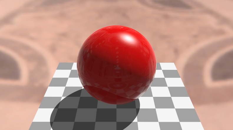
Below is an image of a surface that is degree (2,2). This is a screenshot taken from the interactive webgl2 demo I made for this post: Least Squares Surface Fitting

How Do You Do It?

The two main players from the last post were the ATA matrix and the ATY vector. These two could be incrementally updated as new data points came in, which would allow you to do an incremental (or “online”) least squares fit of a curve.

When working with surfaces and volumes, you have the same things basically. Both the ATA matrix and the ATY vector still exist, but they contain slightly different information – which I’ll explain lower down. However, the ATY vector is renamed, since in the case of a surface it should be called ATZ, and for a volume it should be called ATW. I call it ATV to generalize it, where v stands for value, and represents the last component in a data point, which is the output value we are trying to fit given the input values. The input values are the rest of the components of the data point.

At the end, you once again need to solve the equation A^TA*c=A^Tv to calculate the coefficients (named c) of the equation.

It’s all pretty similar to fitting a curve, but the details change a bit. Let’s work through an example to see how it differs.

Example: Bilinear Surface Fitting

Let’s fit 4 data points to a bilinear surface, otherwise known as a surface that is linear on each axis, or a surface of degree(1,1):
(0,0,5)
(0,1,3)
(1,0,8)
(1,1,2)

Since we are fitting those data points with a bilinear surface, we are looking for a function that takes in x,y values and gives as output the z coordinate. We want a surface that gives us the closest answer possible (minimizing the sum of the squared difference for each input data point) for the data points we do have, so that we can give it other data points and get z values as output that approximate what we expect to see for that input.

A linear equation looks like this, with coefficients A and B:
y=Ax+B

Since we want a bilinear equation this time around, this is the equation we are going to end up with, after solving for the coefficients A,B,C,D:
y=Axy+Bx+Cy+D

The first step is to make the A matrix. In the last post, this matrix was made up of powers of the x coordinates. In this post, they are actually going to be made up of the permutation of powers of the x and y coordinates.

Last time the matrix looked like this:
A =  \begin{bmatrix} x_0^0 & x_0^1 & x_0^2 \\ x_1^0 & x_1^1 & x_1^2 \\ x_2^0 & x_2^1 & x_2^2 \\ x_3^0 & x_3^1 & x_3^2 \\ \end{bmatrix}

This time, the matrix is going to look like this:
A =  \begin{bmatrix} x_0^0y_0^0 & x_0^0y_0^1 & x_0^1y_0^0 & x_0^1y_0^1 \\ x_1^0y_1^0 & x_1^0y_1^1 & x_1^1y_1^0 & x_1^1y_1^1 \\ x_2^0y_2^0 & x_2^0y_2^1 & x_2^1y_2^0 & x_2^1y_2^1 \\ x_3^0y_3^0 & x_3^0y_3^1 & x_3^1y_3^0 & x_3^1y_3^1 \\ \end{bmatrix}

Simplifying that matrix a bit, it looks like this:
A =  \begin{bmatrix} 1 & y_0 & x_0 & x_0y_0 \\ 1 & y_1 & x_1 & x_1y_1 \\ 1 & y_2 & x_2 & x_2y_2 \\ 1 & y_3 & x_3 & x_3y_3 \\ \end{bmatrix}

To simplify it even further, there is one row in the A matrix per data point, where the row looks like this:
\begin{bmatrix} 1 & y & x & xy \\ \end{bmatrix}

You can see that every permutation of the powers of x and y for each data point is present in the matrix.

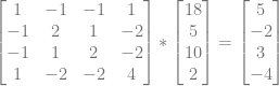
The A matrix for our data points is this:
A =  \begin{bmatrix} 1 & 0 & 0 & 0 \\ 1 & 1 & 0 & 0 \\ 1 & 0 & 1 & 0 \\ 1 & 1 & 1 & 1 \\ \end{bmatrix}

Next we need to calculate the ATA matrix by multiplying the transpose of that matrix, by that matrix.

A^TA =  \begin{bmatrix} 1 & 1 & 1 & 1 \\ 0 & 1 & 0 & 1 \\ 0 & 0 & 1 & 1 \\ 0 & 0 & 0 & 1 \\ \end{bmatrix} * \begin{bmatrix} 1 & 0 & 0 & 0 \\ 1 & 1 & 0 & 0 \\ 1 & 0 & 1 & 0 \\ 1 & 1 & 1 & 1 \\ \end{bmatrix} = \begin{bmatrix} 4 & 2 & 2 & 1 \\ 2 & 2 & 1 & 1 \\ 2 & 1 & 2 & 1 \\ 1 & 1 & 1 & 1 \\ \end{bmatrix}

Taking the inverse of that matrix we get this:

(A^TA)^{-1} =  \begin{bmatrix} 1 & -1 & -1 & 1 \\ -1 & 2 & 1 & -2 \\ -1 & 1 & 2 & -2 \\ 1 & -2 & -2 & 4 \\ \end{bmatrix}

Next we need to calculate the ATV vector (formerly known as ATY). We calculate that by multiplying the transpose of the A matrix by the Z values:

A^TV =  \begin{bmatrix} 1 & 1 & 1 & 1 \\ 0 & 1 & 0 & 1 \\ 0 & 0 & 1 & 1 \\ 0 & 0 & 0 & 1 \\ \end{bmatrix} * \begin{bmatrix} 5 \\ 3 \\ 8 \\ 2 \\ \end{bmatrix} = \begin{bmatrix} 18 \\ 5 \\ 10 \\ 2 \\ \end{bmatrix}

Lastly we multiply the inversed ATA matrix by the ATV vector to get our coefficients.

\begin{bmatrix} 1 & -1 & -1 & 1 \\ -1 & 2 & 1 & -2 \\ -1 & 1 & 2 & -2 \\ 1 & -2 & -2 & 4 \\ \end{bmatrix} * \begin{bmatrix} 18 \\ 5 \\ 10 \\ 2 \\ \end{bmatrix} = \begin{bmatrix} 5 \\ -2 \\ 3 \\ -4 \\ \end{bmatrix}

In the last post, the coefficients we got out were in x power order, so the first (top) was for the x^0 term, the next was for the x^1 term etc.

This time around, the coefficients are in the same order as the permutations of the powers of x and y:
\begin{bmatrix} 1 & y & x & xy \\ \end{bmatrix}

That makes our final equation this:
z = -4xy+3x-2y+5

If you plug in the (x,y) values from the data set we fit, you’ll see that you get the corresponding z values as output. We perfectly fit the data set!

The process isn’t too different from last post and not too difficult either right?

Let’s see if we can generalize and formalize things a bit.

Some Observations

Firstly you may be wondering how we come up with the correct permutation of powers of our inputs. It actually doesn’t matter so long as you are consistent. You can have your A matrix rows have the powers in any order, so long as all orders are present, and you use the same order in all operations.

Regarding storage sizes needed, the storage of surfaces and (hyper) volumes are a bit different and generally larger than curves.

To see how, let’s look at the powers of the ATA matrix of a bilinear surface, using the ordering of powers that we used in the example:

\begin{bmatrix} x^0y^0 & x^0y^1 & x^1y^0 & x^1y^1 \\ x^0y^1 & x^0y^2 & x^1y^1 & x^1y^2 \\ x^1y^0 & x^1y^1 & x^2y^0 & x^2y^1 \\ x^1y^1 & x^1y^2 & x^2y^1 & x^2y^2 \\ \end{bmatrix}

Let’s rewrite it as just the powers:

\begin{bmatrix} 00 & 01 & 10 & 11 \\ 01 & 02 & 11 & 12 \\ 10 & 11 & 20 & 21 \\ 11 & 12 & 21 & 22 \\ \end{bmatrix}

And the permutation we used as just powers to help us find the pattern in the powers of x and y in the ATA matrix:
\begin{bmatrix} 00 & 01 & 10 & 11 \\ \end{bmatrix}

Can you find the pattern of the powers used at the different spots in the ATA matrix?

I had to stare at it for a while before I figured it out but it’s this: For the i,j location in the ATA matrix, the powers of x and y are the powers of x and y in the i permutation added to the powers of x and y in the j permutation.

For example, A^TA_{0,2} has xy powers of 10. Permutation 0 has powers of 0,0 and permutation 2 has powers of 1,0, so we add those together to get powers 1,0.

Another example, A^TA_{2,3} has xy powers of 21. Permutation 2 has powers of 1,0 and permutation 3 has powers 1,1. Adding those together we get 2,1 which is correct.

That’s a bit more complex than last post, not too much more difficult to construct the ATA matrix directly – and also construct it incrementally as new data points come in!

How many unique values are there in the ATA matrix though? We need to know this to know how much storage we need.

In the last post, we needed (degree+1)*2–1 values to store the unique ATA matrix values. That can also be written as degree*2+1.

It turns out that when generalizing this to surfaces and volumes, that we need to take the product of that for each axis.

For instance, a surface has ((degreeX*2)+1)*((degreeY*2)+1) unique values. A volume has ((degreeX*2)+1)*((degreeY*2)+1)*((degreeZ*2)+1) unique values.

The pattern continues for higher dimensions, as well as lower, since you can see how in the curve case, it’s the same formula as it was before.

For the same ATA matrix size, a surface has more unique values than a curve does.

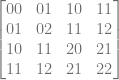
As far as what those values actually are, they are the full permutations of the powers of a surface (or hyper volume) that is one degree higher on each axis. For a bilinear surface, that means the 9 permutations of x and y for powers 0,1 and 2:
x^0y^0,x^0y^1,x^0y^2,x^1y^0,x^1y^1,x^1y^2,x^2y^0,x^2y^1,x^2y^2
Or simplified:
1,y,y^2,x,xy,xy^2,x^2,x^2y,x^2y^2

What about the ATV vector?

For the bilinear case, The ATV vector is the sums of the permutations of x,y multiplied by z, for every data point. In other words, you add this to ATV for each data point:
\begin{bmatrix} z & yz & xz & xyz \\ \end{bmatrix}

How much storage space do we need in general for the ATV vector then? it’s the product of (degree+1) for each axis.

For instance, a surface has (degreeX+1)*(degreeY+1) values in ATV, and a volume has (degreeX+1)*(degreeY+1)*(degreeZ+1).

You may also be wondering how many data points are required minimum to fit a curve, surface or hypervolume to a data set. The answer is that you need as many data points as there are terms in the polynomial. We are trying to solve for the polynomial coefficients, so there are as many unknowns as there are polynomial terms.

How many polynomial terms are there? There are as many terms as there are permutations of the axes powers involved. In other words, the size of ATV is also the minimum number of points you need to fit a curve, surface, or hypervolume to a data set.

Measuring Quality of a Fit

You are probably wondering if there’s a way to calculate how good of a fit you have for a given data set. It turns out that there are a few ways to calculate a value for this.

The value I use in the code below and in the demos is called R^2 or residue squared.

First you calculate the average (mean) output value from the input data set.

Then you calculate SSTot which is the sum of the square of the mean subtracted from each input point’s output value. Pseudo code:

SSTot = 0;
for (point p in points)
  SSTot += (p.out - mean)^2;

You then calculate SSRes which is the sum of the square of the fitted function evaluated at a point, subtracted from each input points’ output value. Pseudo code:

SSRes= 0;
for (point p in points)
  SSRes += (p.out - f(p.in))^2;

The final value for R^2 is 1-SSRes/SSTot.

The value is nice because it’s unitless, and since SSRes and SSTot is a sum of squares, SSRes/SSTot is basically the value that the fitting algorithm minimizes. The value is subtracted from 1 so that it’s a fit quality metric. A value of 0 is a bad fit, and a value of 1 is a good fit and generally it will be between those values.

If you want to read more about this, check out this link: Coefficient of Determination

Example Code

Here is a run from the sample code:

And here is the source code:

#include <stdio.h>
#include <array>

#define FILTER_ZERO_COEFFICIENTS true // if false, will show terms which have a coefficient of 0

//====================================================================
template<size_t N>
using TVector = std::array<float, N>;

template<size_t M, size_t N>
using TMatrix = std::array<TVector<N>, M>;

//====================================================================
// Specify a degree per axis.
// 1 = linear, 2 = quadratic, etc
template <size_t... DEGREES>
class COnlineLeastSquaresFitter
{
public:
    COnlineLeastSquaresFitter ()
    {
        // initialize our sums to zero
        std::fill(m_SummedPowers.begin(), m_SummedPowers.end(), 0.0f);
        std::fill(m_SummedPowersTimesValues.begin(), m_SummedPowersTimesValues.end(), 0.0f);
    }

	// Calculate how many summed powers we need.
	// Product of degree*2+1 for each axis.
	template <class T>
	constexpr static size_t NumSummedPowers(T degree)
	{
		return degree * 2 + 1;
	}
	template <class T, class... DEGREES>
	constexpr static size_t NumSummedPowers(T first, DEGREES... degrees)
	{
		return NumSummedPowers(first) * NumSummedPowers(degrees...);
	}

	// Calculate how many coefficients we have for our equation.
	// Product of degree+1 for each axis.
	template <class T>
	constexpr static size_t NumCoefficients(T degree)
	{
		return (degree + 1);
	}
	template <class T, class... DEGREES>
	constexpr static size_t NumCoefficients(T first, DEGREES... degrees)
	{
		return NumCoefficients(first) * NumCoefficients(degrees...);
	}

	// Helper function to get degree of specific axis
	static size_t Degree (size_t axisIndex)
	{
		static const std::array<size_t, c_dimension-1> c_degrees = { DEGREES... };
		return c_degrees[axisIndex];
	}
	
	// static const values
	static const size_t c_dimension = sizeof...(DEGREES) + 1; 
	static const size_t c_numCoefficients = NumCoefficients(DEGREES...);
	static const size_t c_numSummedPowers = NumSummedPowers(DEGREES...);

	// Typedefs
	typedef TVector<c_numCoefficients> TCoefficients;
	typedef TVector<c_dimension> TDataPoint;

	// Function for converting from an index to a specific power permutation
	static void IndexToPowers (size_t index, std::array<size_t, c_dimension-1>& powers, size_t maxDegreeMultiply, size_t maxDegreeAdd)
	{
		for (int i = c_dimension-2; i >= 0; --i)
		{
			size_t degree = Degree(i) * maxDegreeMultiply + maxDegreeAdd;
			powers[i] = index % degree;
			index = index / degree;
		}
	}

	// Function for converting from a specific power permuation back into an index
	static size_t PowersToIndex (std::array<size_t, c_dimension - 1>& powers, size_t maxDegreeMultiply, size_t maxDegreeAdd)
	{
		size_t ret = 0;
		for (int i = 0; i < c_dimension - 1; ++i)
		{
			ret *= Degree(i) * maxDegreeMultiply + maxDegreeAdd;
			ret += powers[i];
		}
		return ret;
	}

	// Add a datapoint to our fitting
    void AddDataPoint (const TDataPoint& dataPoint)
    {
		// Note: It'd be a good idea to memoize the powers and calculate them through repeated
		// multiplication, instead of calculating them on demand each time, using std::pow.

        // add the summed powers of the input values
		std::array<size_t, c_dimension-1> powers;
        for (size_t i = 0; i < m_SummedPowers.size(); ++i)
        {
			IndexToPowers(i, powers, 2, 1);
			float valueAdd = 1.0;
			for (size_t j = 0; j < c_dimension - 1; ++j)
				valueAdd *= (float)std::pow(dataPoint[j], powers[j]);
			m_SummedPowers[i] += valueAdd;
        }

        // add the summed powers of the input value, multiplied by the output value
        for (size_t i = 0; i < m_SummedPowersTimesValues.size(); ++i)
        {
			IndexToPowers(i, powers, 1, 1);
			float valueAdd = dataPoint[c_dimension - 1];
			for (size_t j = 0; j < c_dimension-1; ++j)
				valueAdd *= (float)std::pow(dataPoint[j], powers[j]);
			m_SummedPowersTimesValues[i] += valueAdd;
        }
    }

	// Get the coefficients of the equation fit to the points
    bool CalculateCoefficients (TCoefficients& coefficients) const
    {
		// make the ATA matrix
		std::array<size_t, c_dimension - 1> powersi;
		std::array<size_t, c_dimension - 1> powersj;
		std::array<size_t, c_dimension - 1> summedPowers;
		TMatrix<c_numCoefficients, c_numCoefficients> ATA;
		for (size_t j = 0; j < c_numCoefficients; ++j)
		{
			IndexToPowers(j, powersj, 1, 1);

			for (size_t i = 0; i < c_numCoefficients; ++i)
			{
				IndexToPowers(i, powersi, 1, 1);

				for (size_t k = 0; k < c_dimension - 1; ++k)
					summedPowers[k] = powersi[k] + powersj[k];

				size_t summedPowersIndex = PowersToIndex(summedPowers, 2, 1);
				ATA[j][i] = m_SummedPowers[summedPowersIndex];
			}
		}

		// solve: ATA * coefficients = m_SummedPowers
		// for the coefficients vector, using Gaussian elimination.
		coefficients = m_SummedPowersTimesValues;
		for (size_t i = 0; i < c_numCoefficients; ++i)
		{
			for (size_t j = 0; j < c_numCoefficients; ++j)
			{
				if (ATA[i][i] == 0.0f)
					return false;

				float c = ((i == j) - ATA[j][i]) / ATA[i][i];
				coefficients[j] += c*coefficients[i];
				for (size_t k = 0; k < c_numCoefficients; ++k)
					ATA[j][k] += c*ATA[i][k];
			}
		}

		// Note: this is the old, "bad" way to solve the equation using matrix inversion.
		// It's a worse choice for larger matrices, and surfaces and volumes use larger matrices than curves in general.
		/*
		// Inverse the ATA matrix
		TMatrix<c_numCoefficients, c_numCoefficients> ATAInverse;
		if (!InvertMatrix(ATA, ATAInverse))
			return false;

		// calculate the coefficients
		for (size_t i = 0; i < c_numCoefficients; ++i)
			coefficients[i] = DotProduct(ATAInverse[i], m_SummedPowersTimesValues);
		*/

		return true;
    }

private:
	//Storage Requirements:
	// Summed Powers = Product of degree*2+1 for each axis.
	// Summed Powers Times Values = Product of degree+1 for each axis.
    TVector<c_numSummedPowers>		m_SummedPowers;
	TVector<c_numCoefficients>		m_SummedPowersTimesValues;
};

//====================================================================
char AxisIndexToLetter (size_t axisIndex)
{
	// x,y,z,w,v,u,t,....
	if (axisIndex < 3)
		return 'x' + char(axisIndex);
	else
		return 'x' + 2 - char(axisIndex);
}

//====================================================================
template <class T, size_t M, size_t N>
float EvaluateFunction (const T& fitter, const TVector<M>& dataPoint, const TVector<N>& coefficients)
{
	float ret = 0.0f;
	for (size_t i = 0; i < coefficients.size(); ++i)
	{
		// start with the coefficient
		float term = coefficients[i];

		// then the powers of the input variables
		std::array<size_t, T::c_dimension - 1> powers;
		fitter.IndexToPowers(i, powers, 1, 1);
		for (size_t j = 0; j < powers.size(); ++j)
			term *= (float)std::pow(dataPoint[j], powers[j]);

		// add this term to our return value
		ret += term;
	}
	return ret;
}

//====================================================================
template <size_t... DEGREES>
void DoTest (const std::initializer_list<TVector<sizeof...(DEGREES)+1>>& data)
{
	// say what we are are going to do
	printf("Fitting a function of degree (");
	for (size_t i = 0; i < COnlineLeastSquaresFitter<DEGREES...>::c_dimension - 1; ++i)
	{
		if (i > 0)
			printf(",");
		printf("%zi", COnlineLeastSquaresFitter<DEGREES...>::Degree(i));
	}
	printf(") to %zi data points: n", data.size());

	// show input data points
	for (const COnlineLeastSquaresFitter<DEGREES...>::TDataPoint& dataPoint : data)
	{
		printf("  (");
		for (size_t i = 0; i < dataPoint.size(); ++i)
		{
			if (i > 0)
				printf(", ");
			printf("%0.2f", dataPoint[i]);
		}
		printf(")n");
	}

	// fit data
	COnlineLeastSquaresFitter<DEGREES...> fitter;
    for (const COnlineLeastSquaresFitter<DEGREES...>::TDataPoint& dataPoint : data)
        fitter.AddDataPoint(dataPoint);

	// calculate coefficients if we can
	COnlineLeastSquaresFitter<DEGREES...>::TCoefficients coefficients;
	bool success = fitter.CalculateCoefficients(coefficients);
	if (!success)
	{
		printf("Could not calculate coefficients!nn");
		return;
	}

	// print the polynomial
	bool firstTerm = true;
	printf("%c = ", AxisIndexToLetter(sizeof...(DEGREES)));
    bool showedATerm = false;
	for (int i = (int)coefficients.size() - 1; i >= 0; --i)
	{
		// don't show zero terms
		if (FILTER_ZERO_COEFFICIENTS && std::abs(coefficients[i]) < 0.00001f)
			continue;

        showedATerm = true;

		// show an add or subtract between terms
		float coefficient = coefficients[i];
		if (firstTerm)
			firstTerm = false;
		else if (coefficient >= 0.0f)
			printf(" + ");
		else
		{
			coefficient *= -1.0f;
			printf(" - ");
		}

		printf("%0.2f", coefficient);

		std::array<size_t, COnlineLeastSquaresFitter<DEGREES...>::c_dimension - 1> powers;
		fitter.IndexToPowers(i, powers, 1, 1);

		for (size_t j = 0; j < powers.size(); ++j)
		{
			if (powers[j] > 0)
				printf("%c", AxisIndexToLetter(j));
			if (powers[j] > 1)
				printf("^%zi", powers[j]);
		}
	}
    if (!showedATerm)
        printf("0");
	printf("n");

	// Calculate and show R^2 value.
	float rSquared = 1.0f;
	if (data.size() > 0)
	{
		float mean = 0.0f;
		for (const COnlineLeastSquaresFitter<DEGREES...>::TDataPoint& dataPoint : data)
			mean += dataPoint[sizeof...(DEGREES)];
		mean /= data.size();
		float SSTot = 0.0f;
		float SSRes = 0.0f;
		for (const COnlineLeastSquaresFitter<DEGREES...>::TDataPoint& dataPoint : data)
		{
			float value = dataPoint[sizeof...(DEGREES)] - mean;
			SSTot += value*value;

			value = dataPoint[sizeof...(DEGREES)] - EvaluateFunction(fitter, dataPoint, coefficients);
			SSRes += value*value;
		}
		if (SSTot != 0.0f)
			rSquared = 1.0f - SSRes / SSTot;
	}
	printf("R^2 = %0.4fnn", rSquared);
}

//====================================================================
int main (int argc, char **argv)
{
	// bilinear - 4 data points
	DoTest<1, 1>(
		{
			TVector<3>{ 0.0f, 0.0f, 5.0f },
			TVector<3>{ 0.0f, 1.0f, 3.0f },
			TVector<3>{ 1.0f, 0.0f, 8.0f },
			TVector<3>{ 1.0f, 1.0f, 2.0f },
		}
	);

	// biquadratic - 9 data points
	DoTest<2, 2>(
		{
			TVector<3>{ 0.0f, 0.0f, 8.0f },
			TVector<3>{ 0.0f, 1.0f, 4.0f },
			TVector<3>{ 0.0f, 2.0f, 6.0f },
			TVector<3>{ 1.0f, 0.0f, 5.0f },
			TVector<3>{ 1.0f, 1.0f, 2.0f },
			TVector<3>{ 1.0f, 2.0f, 1.0f },
			TVector<3>{ 2.0f, 0.0f, 7.0f },
			TVector<3>{ 2.0f, 1.0f, 9.0f },
			TVector<3>{ 2.0f, 2.5f, 12.0f },
		}
	);

	// trilinear - 8 data points
	DoTest<1, 1, 1>(
		{
			TVector<4>{ 0.0f, 0.0f, 0.0f, 8.0f },
			TVector<4>{ 0.0f, 0.0f, 1.0f, 4.0f },
			TVector<4>{ 0.0f, 1.0f, 0.0f, 6.0f },
			TVector<4>{ 0.0f, 1.0f, 1.0f, 5.0f },
			TVector<4>{ 1.0f, 0.0f, 0.0f, 2.0f },
			TVector<4>{ 1.0f, 0.0f, 1.0f, 1.0f },
			TVector<4>{ 1.0f, 1.0f, 0.0f, 7.0f },
			TVector<4>{ 1.0f, 1.0f, 1.0f, 9.0f },
		}
	);

	// trilinear - 9 data points
	DoTest<1, 1, 1>(
		{
			TVector<4>{ 0.0f, 0.0f, 0.0f, 8.0f },
			TVector<4>{ 0.0f, 0.0f, 1.0f, 4.0f },
			TVector<4>{ 0.0f, 1.0f, 0.0f, 6.0f },
			TVector<4>{ 0.0f, 1.0f, 1.0f, 5.0f },
			TVector<4>{ 1.0f, 0.0f, 0.0f, 2.0f },
			TVector<4>{ 1.0f, 0.0f, 1.0f, 1.0f },
			TVector<4>{ 1.0f, 1.0f, 0.0f, 7.0f },
			TVector<4>{ 1.0f, 1.0f, 1.0f, 9.0f },
			TVector<4>{ 0.5f, 0.5f, 0.5f, 12.0f },
		}
	);

	// Linear - 2 data points
    DoTest<1>(
        {
            TVector<2>{ 1.0f, 2.0f },
            TVector<2>{ 2.0f, 4.0f },
        }
    );

	// Quadratic - 4 data points
    DoTest<2>(
        {
            TVector<2>{ 1.0f, 5.0f },
			TVector<2>{ 2.0f, 16.0f },
			TVector<2>{ 3.0f, 31.0f },
			TVector<2>{ 4.0f, 16.0f },
        }
    );

	// Cubic - 4 data points
    DoTest<3>(
        {
            TVector<2>{ 1.0f, 5.0f },
            TVector<2>{ 2.0f, 16.0f },
			TVector<2>{ 3.0f, 31.0f },
			TVector<2>{ 4.0f, 16.0f },
        }
    );

    system("pause");
    return 0;
}

Closing

The next logical step here for me would be to figure out how to break the equation for a surface or hypervolume up into multiple equations, like you’d have with a tensor product surface/hypervolume equation. It would also be interesting to see how to convert from these multidimensional polynomials to multidimensional Bernstein basis functions, which are otherwise known as Bezier rectangles (and Bezier hypercubes i guess).

The last post inverted the ATA matrix and multiplied by ATY to get the coefficients. Thanks to some feedback on reddit, I found out that is NOT how you want to solve this sort of equation. I ended up going with Gaussian elimination for this post which is more numerically robust while also being less computation to calculate. There are other options out there too that may be even better choices. I’ve found out that in general, if you are inverting a matrix in code, or even just using an inverted matrix that has already been given to you, you are probably doing it wrong. You can read more about that here: John D. Cook: Don’t invert that matrix.

I didn’t go over what to do if you don’t have enough data points because if you find yourself in that situation, you can either decrease the degree of one of the axes, or you could remove and axis completely if you wanted to. It’s situational and ambiguous what parameter to decrease when you don’t have enough data points to fit a specific curve or hypervolume, but it’s still possible to decay the fit to a lower degree or dimension if you hit this situation, because you will already have all the values you need in the ATA matrix values and the ATV vector. I leave that to you to decide how to handle it in your own usage cases. Something interesting to note is that ATA[0][0] is STILL the count of how many data points you have, so you can use this value to know how much you need to decay your fit to be able to handle the data set.

In the WebGL2 demo I mention, I use a finite difference method to calculate the normals of the surface, however since the surface is described by a polynomial, it’d be trivial to calculate the coefficients for the equations that described the partial derivatives of the surface for each axis and use those instead.

I also wanted to mention that in the case of surfaces and hypervolumes it’s still possible to get an imperfect fit to your data set, even though you may give the exact minimum required number of control points. The reason for this is that not all axes are necesarily created equal. If you have a surface of degree (1,2) it’s linear on the x axis, but quadratic on the y axis, and requires a minimum of 6 data points to be able to fit a data set. As you can imagine, it’s possible to give data points such that the data points ARE NOT LINEAR on the x axis. When this happens, the surface will not be a perfect fit.

Lastly, you may be wondering how to fit data sets where there is more than one output value, like an equation of the form
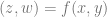
 (z,w)=f(x,y).

I’m not aware of any ways to least square fit that as a whole, but apparently a common practice is to fit one equation to z and another to w and treat them independently. There is a math stack exchange question about that here: Math Stack Exchange: Least square fitting multiple values

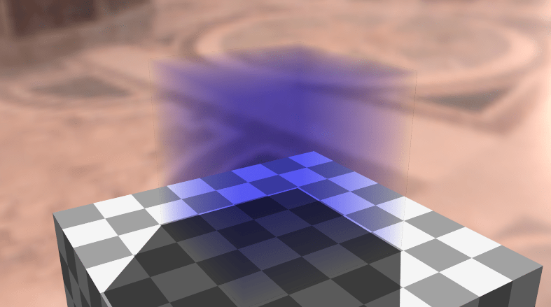
Here is the webgl demo that goes with this post again:
Least Squares Surface Fitting

Thanks for reading, and please speak up if you have anything to add or correct, or a comment to make!