August « 2016 « The blog at the bottom of the sea

I’ve been working on getting a better understanding of the Discrete Fourier Transform. I’ve figured out some things which have really helped my intuition, and made it a lot simpler in my head, so I wanted to write these up for the benefit of other folks, as well as for my future self when I need a refresher.

The discrete Fourier transform takes in data and gives out the frequencies that the data contains. This is useful if you want to analyze data, but can also be useful if you want to modify the frequencies then use the inverse discrete Fourier transform to generate the frequency modified data.

Multiplying By Sinusoids (Sine / Cosine)

If you had a stream of data that had a single frequency in it at a constant amplitude, and you wanted to know the amplitude of that frequency, how could you figure that out?

One way would be to make a cosine wave of that frequency and multiply each sample of your wave by the corresponding samples.

For instance, let’s say that we have a data stream of four values that represent a 1hz cosine wave: 1, 0, -1, 0.

We could then multiply each point by a corresponding point on a cosine wave, add sum them together:

We get.. 1*1 + 0*0 + -1*-1 + 0*0 = 2.

The result we get is 2, which is twice the amplitude of the data points we had. We can divide by two to get the real amplitude.

To show that this works for any amplitude, here’s the same 1hz cosine wave data with an amplitude of five: 5, 0, -5, 0.

Multiplying by the 1hz cosine wave, we get… 5*1 + 0*0 + -5*-1 + 0*0 = 10.

The actual amplitude is 5, so we can see that our result was still twice the amplitude.

In general, you will need to divide by N / 2 where N is the number of samples you have.

What happens if our stream of data has something other than a cosine wave in it though?

Let’s try a sine wave: 0, 1, 0, -1

When we multiply those values by our cosine wave values we get: 0*1 + 1*0 + 0*-1 + -1*0 = 0.

We got zero. Our method broke!

In this case, if instead of multiplying by cosine, we multiply by sine, we get what we expect: 0*0 + 1*1 + 0*0 + -1*-1 = 2. We get results consistent with before, where our answer is the amplitude times two.

That’s not very useful if we have to know whether we are looking for a sine or cosine wave though. We might even have some other type of wave that is neither one!

The solution to this problem is actually to multiply the data points by both cosine and sine waves, and keep both results.

Let’s see how that works.

For this example We’ll take a cosine wave and shift it 0.25 radians to give us samples: 0.97, -0.25, -0.97, 0.25. (The formula is cos(x*2*pi/4+0.25) from 0 to 3)

When we multiply that by a cosine wave we get: 0.97*1 + -0.25*0 + -0.97*-1 + 0.25*0 = 1.94
When we multiply it by a sine wave we get: 0.97*0 + -0.25*1 + -0.97*0 + 0.25*-1 = -0.5

Since we know both of those numbers are twice the actual amplitude, we can divide them both by two to get:
cosine: 0.97
sine: -0.25

Those numbers kind of makes sense if you think about it. We took a cosine wave and shifted it over a little bit so our combined answer is that it’s mostly a cosine wave, but is heading towards being a sine wave (technically a sine wave that has an amplitude of -1, so is a negative sine wave, but is still a sine wave).

To get the amplitude of our phase shifted wave, we treat those values as a vector, and get the magnitude. sqrt((0.97*0.97)+(-0.25*-0.25)) = 1.00. That is correct! Our wave’s amplitude is 1.0.

To get the starting angle (phase) of the wave, we use inverse tangent of sine over cosine. We want to take atan2(sine, cosine), aka atan2(-0.25, 0.97) which gives us a result of -0.25 radians. That’s the amount that we shifted our wave, so it is also correct!

Formulas So Far

Let’s take a look at where we are at mathematically. For $N$ samples of data, we multiply each sample of data by a sample from a wave with the frequency we are looking for and sum up the results (Note that this is really just a dot product between N dimensional vectors!). We have to do this both with a cosine wave and a sine wave, and keep the two resulting values to be able to get our true amplitude and phase information.

For now, let’s drop the “divide by two” part and look at the equations we have.

$Value_{cosine} = \sum\limits_{n=0}^{N-1} Sample_n * Cos(2\pi*Frequency*n/N)$

$Value_{sine} = \sum\limits_{n=0}^{N-1} Sample_n * Sin(2\pi*Frequency*n/N)$

Those equations above do exactly what we worked through in the samples.

The part that might be confusing is the part inside of the Cos() and Sin() so I’ll explain that real quick.

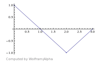
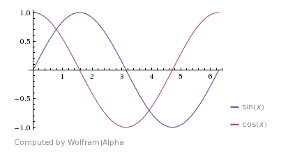
Looking at the graph cos(x) and sin(x) you’ll see that they both make one full cycle between the x values of 0 and 2*pi (aprox. 6.28):

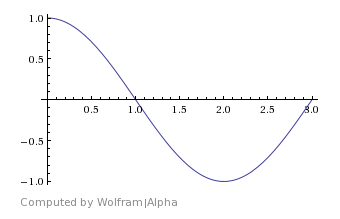
If instead we change it to a graph of cos(2*pi*x) and sin(2*pi*x) you’ll notice that they both make one full cycle between the x values of 0 and 1:

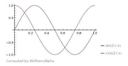
This means that we can think of the wave forms in terms of percent (0 to 1) instead of in radians (0 to 2pi).

Next, we multiply by the frequency we are looking for. We do this because that multiplication makes the wave form repeat that many times between 0 and 1. It makes us a wave of the desired frequency, still remaining in “percent space” where we can go from 0 to 1 to get samples on our cosine and sine waves.

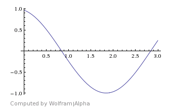
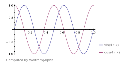
Here’s a graph of cos(2*pi*x*2) and sin(2*pi*x*2), to show some 2hz frequency waves:

Lastly, we multiply by n/N. In our sum, n is our index variable and it goes from 0 to N-1. This is very much like a for loop. n/N is our current percent done we are in the for loop, so when we multiply by n/N, we are just sampling at a different location (by percentage done) on our cosine and sine waves that are at the specified frequencies.

Not too difficult right?

Imaginary Numbers

Wouldn’t it be neat if instead of having to do two separate calculations for our cosine and sine values, we could just do a single calculation that would give us both values?

Well, interestingly, we can! This is where imaginary numbers come in. Don’t get scared, they are here to make things simpler and more convenient, not to make things more complicated or harder to understand (:

There is something called Euler’s Identity which states the below:

$e^{ix} = cos(x) + i*sin(x)$

That looks pretty useful for our usage case doesn’t it? If you notice that our equations both had the same parameters for cos and sin, that means that we can just use this identity instead!

We can now take our two equations and combine them into a single equation:

$Value = \sum\limits_{n=0}^{N-1} Sample_n * e^{i *2\pi * Frequency*n/N}$

When we do the above calculation, we will get a complex number out with a real and imaginary part. The real part of the complex number is just the cosine value, while the imaginary part of the complex number is the sine value. Nothing scary has happened, we’ve just used/abused complex numbers a bit to give us what we want in a more compact form.

Multiple Frequencies

Now we know how to look for a single, specific frequency.

What if you want to look for multiple frequencies though? Further more, what if you don’t even know what frequencies to look for?

When doing the discrete Fourier transform on a stream of samples, there are a specific set of frequencies that it checks for. If you have N samples, it only checks for N different frequencies. You could ask about other frequencies, but these frequencies are enough to reconstruct the original signal from only the frequency data.

The first N/2 frequencies are going to be the frequencies 0 (DC) through N/2. N/2 is the Nyquist frequency and is the highest frequency that your signal is able of holding.

After N/2 comes the negative frequencies, counting from a large negative frequency (N/2-1) up to the last frequency which is -1.

As an example, if you had 8 samples and ran the DFT, you’d get 8 complex numbers as outputs, which represent these frequencies:

[0hz, 1hz, 2hz, 3hz, 4hz, -3hz, -2hz, -1hz]

The important take away from this section is that if you have N samples, the DFT asks only about N very specific frequencies, which will give enough information to go from frequency domain back to time domain and get the signal data back.

That then leads to this equation below, where we just put a subscript on Value, to signify which frequency we are probing for.

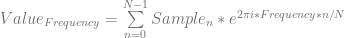
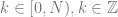
$Value_{Frequency} = \sum\limits_{n=0}^{N-1} Sample_n * e^{2\pi i*Frequency*n/N}$

Frequency is an integer, and is between 0 and N-1. We can say that mathematically by listing this information along with the equation:

$Frequency \in [0,N), Frequency \in \mathbb Z$

Final Form

Math folk use letters and symbols instead of words in their equations.

The letter $k$ is used instead of frequency.

Instead of $Value_{Frequency}$ , the symbol is $X_{k}$ .

Instead of $Sample_n$ , the symbol is $x_n$ .

This gives us a more formal version of the equation:

$X_k= \sum\limits_{n=0}^{N-1} x_n * e^{2\pi ikn/N}$

$k\in [0,N), k \in \mathbb Z$

We are close to the final form, but we aren’t quite done yet!

Remember the divide by two? I had us take out the divide by two so that I could re-introduce it now in it’s correct form. Basically, since we are querying for N frequencies, we need to divide each frequency’s result by N. I mentioned that we had to divide by N/2 to make the amplitude information correct, but since we are checking both positive AND negative frequencies, we have to divide by 2*(N/2), or just N. That makes our equation become this:

$X_k= 1/N \sum\limits_{n=0}^{N-1} x_n * e^{2\pi ikn/N}$

$k\in [0,N), k \in \mathbb Z$

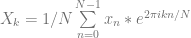
Lastly, we actually want to make the waves go backwards, so we make the exponent negative. The reason for this is a deeper topic than I want to get into right now, but you can read more about why here if you are curious: DFT – Why are the definitions for inverse and forward commonly switched?

That brings us to our final form of the formula for the discrete Fourier transform:

$X_k= 1/N \sum\limits_{n=0}^{N-1} x_n * e^{-2\pi ikn/N}$

$k\in [0,N), k \in \mathbb Z$

Taking a Test Drive

If we use that formula to calculate the DFT of a simple, 4 sample, 1hz cosine wave (1, 0, -1, 0), we get as output [0, 0.5, 0, -0.5].

That means the following:

0hz : 0 amplitude
1hz : 0.5 amplitude
2hz : 0 amplitude
-1hz : -0.5 amplitude

It is a bit strange that the simple 1hz, 1.0 amplitude cosine wave was split in half, and made into a 1hz cosine wave and -1hz cosine wave, each contributing half amplitude to the result, but that is “just how it works”. I don’t have a very good explanation for this though. My personal understanding just goes that if we are checking for both positive AND negative frequencies, that makes it ambiguous whether it’s a 1hz wave with 1 amplitude, or -1hz wave with -1 amplitude. Since it’s ambiguous, both must be true, and they get half the amplitude each. If I get a better understanding, I’ll update this paragraph, or make a new post on it.

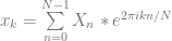
Making The Inverse Discrete Fourier Transform

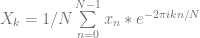
Making the formula for the Inverse DFT is really simple.

We start with our DFT formula, drop the 1/N from the front, and also make the exponent to e positive instead of negative. That is all! The intuition here for me is that we are just doing the reverse of the DFT process, to do the inverse DFT process.

$x_k= \sum\limits_{n=0}^{N-1} X_n * e^{2\pi ikn/N}$

$k\in [0,N), k \in \mathbb Z$

While the DFT takes in real valued signals and gives out complex valued frequency data, the IDFT takes in complex valued frequency data, and gives out real valued signals.

A fun thing to try is to take some data, DFT it, modify the frequency data, then IDFT it to see what comes out the other side.

Other Notes

Here are some other things of note about the discrete Fourier transform and it’s inverse.

Data Repeating Forever

When you run the DFT on a stream of data, the math is such that it assumes that the stream of data you gave it repeats forever both forwards and backwards in time. This is important because if you aren’t careful, you can add frequency content to your data that you didn’t intend to be there.

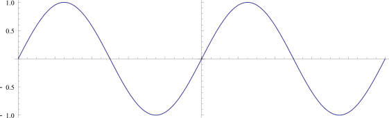
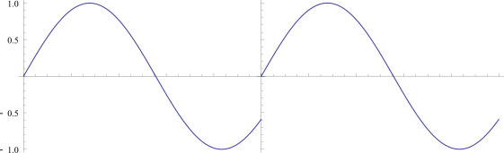
For instance, if you tile a 1hz sine wave, it’s continuous, and there is only the 1hz frequency present:

However, if you tile a 0.9hz sine wave, there is a discontinuity, which means that there will be other, unintended frequencies present when you do a DFT of the data, to be able to re-create the discontinuity:

Fast Fourier Transform

There are a group of algorithms called “Fast Fourier Transforms”. You might notice that if we have N samples, taking the DFT is an O(N^2) operation. Fast Fourier transforms can bring it down to O(N log N).

DFT / IDFT Formula Variations

The formula we came up with is one possible DFT formula, but there are a handful of variations that are acceptable, even though different variations come up with different values!

The first option is whether to make the e exponent negative or not. Check out these two formulas to see what I mean.

$X_k= \sum\limits_{n=0}^{N-1} x_n * e^{2\pi ikn/N}$
vs
$X_k= \sum\limits_{n=0}^{N-1} x_n * e^{-2\pi ikn/N}$

Either one is acceptable, but when providing DFT’d data, you should mention which one you did, and make sure and use the opposite one in your inverse DFT formula.

The next options is whether to divide by N or not, like the below:

$X_k= \sum\limits_{n=0}^{N-1} x_n * e^{2\pi ikn/N}$
vs
$X_k= 1/N \sum\limits_{n=0}^{N-1} x_n * e^{2\pi ikn/N}$

Again, either one is acceptable, but you need to make sure and let people know which one you did, and also make sure and use the opposite one in your inverse DFT formula.

Instead of dividing by N, some people actually divide by 1/sqrt(N) in both the DFT and inverse DFT. Wolfram alpha does this for instance!

You can read more about this stuff here: DFT – Why are the definitions for inverse and forward commonly switched?

One thing to note though is that if doing 1/N on the DFT (my personal preference), the 0hz (DC) frequency bin gives you the average value of the signal, and the amplitude data you get out of the other bins is actually correct (keeping in mind the amplitudes are split in half between positive and negative frequencies).

Why Calculate Negative Frequencies

The negative frequencies are able to be calculated on demand from the positive frequency information (eg complex conjugation), so why should we even bother calculating them? Sure it’d be more computationally efficient not to calculate them, especially when just doing frequency analysis, right?!

Here’s a discussion about that: Why calculate negative frequencies of DFT?

Higher Dimensions

It’s possible to DFT in 2d, 3d, and higher. The last blog post shows how to do this with 2d images, but I’d also like to write a blog post like this one specifically talking about the intuition behind multi dimensional DFTs.

Example Program Source Code

Here’s some simple C++ source code which calculates the DFT and inverse DFT, optionally showing work in case you want to try to work some out by hand to better understand this. Working a few out by hand really helped me get a better intuition for all this stuff.

Program Output:

Source Code:

#include <stdio.h>
#include <complex>
#include <vector>

#include <fcntl.h>
#include <io.h>
 
// set to 1 to have it show you the steps performed.  Set to 0 to hide the work.
// useful if checking work calculated by hand.
#define SHOW_WORK 1
 
#if SHOW_WORK
    #define PRINT_WORK(...) wprintf(__VA_ARGS__)
#else
    #define PRINT_WORK(...)
#endif

// Use UTF-16 encoding for Greek letters
static const wchar_t kPi = 0x03C0;
static const wchar_t kSigma = 0x03A3;
 
typedef float TRealType;
typedef std::complex<TRealType> TComplexType;
 
const TRealType c_pi = (TRealType)3.14159265359;
const TRealType c_twoPi = (TRealType)2.0 * c_pi;
 
//=================================================================================
TComplexType DFTSample (const std::vector<TRealType>& samples, int k)
{
    size_t N = samples.size();
    TComplexType ret;
    for (size_t n = 0; n < N; ++n)
    {
        TComplexType calc = TComplexType(samples[n], 0.0f) * std::polar<TRealType>(1.0f, -c_twoPi * TRealType(k) * TRealType(n) / TRealType(N));
        PRINT_WORK(L"    n = %i : (%f, %f)n", n, calc.real(), calc.imag());
        ret += calc;
    }
    ret /= TRealType(N);
    PRINT_WORK(L"    Sum the above and divide by %in", N);
    return ret;
}
 
//=================================================================================
std::vector<TComplexType> DFTSamples (const std::vector<TRealType>& samples)
{
    PRINT_WORK(L"DFT:  X_k = 1/N %cn[0,N) x_k * e^(-2%cikn/N)n", kSigma, kPi);
 
    size_t N = samples.size();
    std::vector<TComplexType> ret;
    ret.resize(N);
    for (size_t k = 0; k < N; ++k)
    {
        PRINT_WORK(L"  k = %in", k);
        ret[k] = DFTSample(samples, k);
        PRINT_WORK(L"  X_%i = (%f, %f)n", k, ret[k].real(), ret[k].imag());
    }
    PRINT_WORK(L"n");
    return ret;
}
 
//=================================================================================
TRealType IDFTSample (const std::vector<TComplexType>& samples, int k)
{
    size_t N = samples.size();
    TComplexType ret;
    for (size_t n = 0; n < N; ++n)
    {
        TComplexType calc = samples[n] * std::polar<TRealType>(1.0f, c_twoPi * TRealType(k) * TRealType(n) / TRealType(N));
        PRINT_WORK(L"    n = %i : (%f, %f)n", n, calc.real(), calc.imag());
        ret += calc;
    }
    PRINT_WORK(L"    Sum the above and take the real componentn");
    return ret.real();
}
 
//=================================================================================
std::vector<TRealType> IDFTSamples (const std::vector<TComplexType>& samples)
{
    PRINT_WORK(L"IDFT:  x_k = %cn[0,N) X_k * e^(2%cikn/N)n", kSigma, kPi);
 
    size_t N = samples.size();
    std::vector<TRealType> ret;
    ret.resize(N);
    for (size_t k = 0; k < N; ++k)
    {
        PRINT_WORK(L"  k = %in", k);
        ret[k] = IDFTSample(samples, k);
        PRINT_WORK(L"  x_%i = %fn", k, ret[k]);
    }
    PRINT_WORK(L"n");
    return ret;
}
 
//=================================================================================
template<typename LAMBDA>
std::vector<TRealType> GenerateSamples (int numSamples, LAMBDA lambda)
{
    std::vector<TRealType> ret;
    ret.resize(numSamples);
    for (int i = 0; i < numSamples; ++i)
    {
        TRealType percent = TRealType(i) / TRealType(numSamples);
        ret[i] = lambda(percent);
    }
    return ret;
}
 
//=================================================================================
int main (int argc, char **argv)
{
	// Enable Unicode UTF-16 output to console
	_setmode(_fileno(stdout), _O_U16TEXT);

    // You can test specific data samples like this:
    //std::vector<TRealType> sourceData = { 1, 0, 1, 0 }; 
    //std::vector<TRealType> sourceData = { 1, -1, 1, -1 };
 
    // Or you can generate data samples from a function like this
    std::vector<TRealType> sourceData = GenerateSamples(
        4,
        [] (TRealType percent)
        {
            const TRealType c_frequency = TRealType(1.0);
            return cos(percent * c_twoPi * c_frequency);
        }
    );
 
    // Show the source data
    wprintf(L"nSource = [ ");
    for (TRealType v : sourceData)
        wprintf(L"%f ",v);
    wprintf(L"]nn");
 
    // Do a dft and show the results
    std::vector<TComplexType> dft = DFTSamples(sourceData);
    wprintf(L"dft = [ ");
    for (TComplexType v : dft)
        wprintf(L"(%f, %f) ", v.real(), v.imag());
    wprintf(L"]nn");
 
    // Do an inverse dft of the dft data, and show the results
    std::vector<TRealType> idft = IDFTSamples(dft);
    wprintf(L"idft = [ ");
    for (TRealType v : idft)
        wprintf(L"%f ", v);
    wprintf(L"]n");
     
    return 0;
}

Links

Explaining how to calculate the frequencies represented by the bins of output of DFT:
How do I obtain the frequencies of each value in an FFT?

Another good explanation of the Fourier transform if it isn’t quite sinking in yet:
An Interactive Guide To The Fourier Transform

Some nice dft calculators that also have inverse dft equivelants:
DFT Calculator 1
IDFT Calculator 1
DFT Calculator 2
IDFT Calculator 2

Wolfram alpha can also do DFT and IDFT, but keep in mind that the formula used there is different and divides the results by 1/sqrt(N) in both DFT and IDFT so will be different values than you will get if you use a different formula.

Wolfram Alpha: Fourier[{1, 0, -1, 0}] = [0,1,0,1]

Wolfram Alpha: Inverse Fourier[{0, 1 , 0, 1}] = [1, 0, -1, 0]

The blog at the bottom of the sea

Programming, Graphics, Gamedev, Exotic Computation, Audio Synthesis

Monthly Archives: August 2016

Incremental Averaging

Understanding The Discrete Fourier Transform

Multiplying By Sinusoids (Sine / Cosine)

Formulas So Far

Imaginary Numbers

Multiple Frequencies

Final Form

Taking a Test Drive

Making The Inverse Discrete Fourier Transform

Other Notes

Example Program Source Code

Links