
The last post showed how to transform uniformly generated random numbers into any random number distribution you desired.
It did so by turning the PDF (probability density function) into a CDF (cumulative density function) and then inverting it – either analytically (making a function) or numerically (making a look up table).
This post will show you how to generate numbers from a PDF as well, but will do so using rejection sampling.
Dice
Let’s say you wanted to simulate a fair five sided die but that you only had a six sided die.
You can use rejection sampling for this by rolling a six sided die and ignoring the roll any time a six came up. Doing that, you do in fact get a fair five sided die roll!
This shows doing that to get 10,000 five sided die rolls:
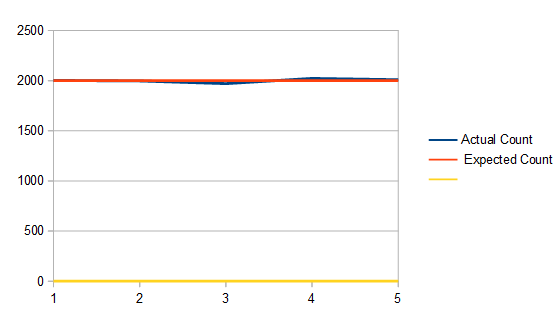
One disadvantage to this method is that you are throwing away die rolls which can be a source of inefficiency. In this setup it takes 1.2 six sided die rolls on average to get a valid five sided die roll since a roll will be thrown away 1/6 of the time.
Another disadvantage is that each time you need a new value, there are an unknown number of die rolls needed to get it. On average it’s true that you only need 1.2 die rolls, but in reality, it’s possible you may roll 10 sixes in a row. Heck it’s even technically possible (but very unlikely) that you could be rolling dice until the end of time and keep getting sixes. (Using PRNG’s in computers, this won’t happen, but it does take a variable number of rolls).
This is just to say: there is uneven and unpredictable execution time of this algorithm, and it needs an unknown (but somewhat predictable) amount of random numbers to work. This is true of the other forms of sampling methods I talk about lower down as well.
Instead of using a six sided die you could use a die of any size that is greater than (or equal to…) five. Here shows a twenty sided die simulating a five sided die:
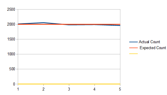
It looks basically the same as using a six sided die, which makes sense (that shows that it works), but in this case, it actually took 4 rolls on average to make a valid five sided die roll, since the roll fails 15/20 times (3 out of 4 rolls will fail).
Quick Asides:
- If straying from rejection sampling ideas for a minute, in the case of the twenty sided die, you could use modulus to get a fair five sided die roll each time:
. This works because there is no remainder for 20 % 5. If there was a remainder it would bias the rolls towards the numbers <= the remainder, making them more likely to come up than the other numbers.
- You could also get a four sided die roll at the same time if you didn’t want to waste any of this precious random information:
- Another algorithm to check out for discrete (integer) weighted random numbers is Vose’s method: Vose’s Method.

Box Around PDF
Moving back into the world of continuous valued random numbers and PDF’s, a simple version of how rejection sampling can be used is like this:
- Graph your PDF
- Draw a box around the PDF
- Generate a (uniform) random point in that box
- If the point is under the curve of the PDF, use the x axis value as your random number, else throw it out and go to 1
That’s all there is to it!
This works because the x axis value of your 2d point is the random number you might be choosing. The y axis value of your 2d point is a probability of choosing that point. Since the PDF graph is higher in places that are more probable, those places are more likely to accept your 2d point than places that have lower PDF values.
Furthermore, the average number of rejected samples vs accepted samples is based on the area under the PDF compared to the area of the box.
The number of samples on average will be the area of the box divided by the area of the PDF.
Since PDF’s by definition have to integrate to 1, that means that you are dividing by 1. So, to simplify: The number of samples on average will be the same as the area of the box!
If it’s hard to come up with the exact size of the box for the PDF, the box doesn’t have to fit exactly, but of course the tighter you can fit the box around the PDF, the fewer rejected samples you’ll have.
You don’t actually need to graph the PDF and draw a box to do this though. Just generate a 2d random number (a random x and a random y) and reject the point if 
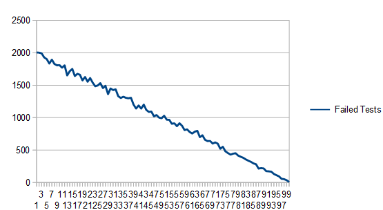
Here I'm using this technique with the PDF 
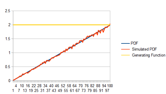
As expected, it took on average 2 points to get a single valid point since the area of the box is 2. Here are how many failed tests each histogram bucket had. Unsurprisingly, lower values of the PDF have more failed tests!
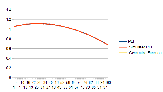
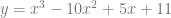
Moving to a more complex PDF, let’s look at
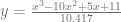
Here are 10 million samples (lots of samples to minimize the noise), using a box height of 1.2, which unsurprisingly takes 1.2 samples on average to get a valid sample:
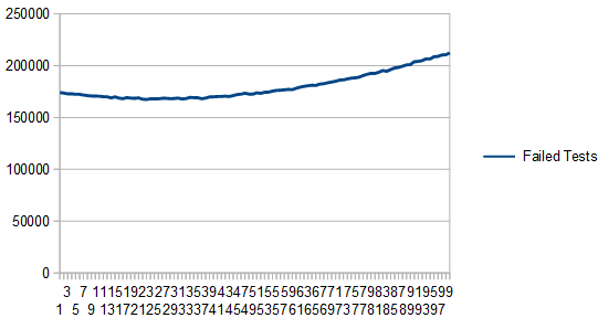
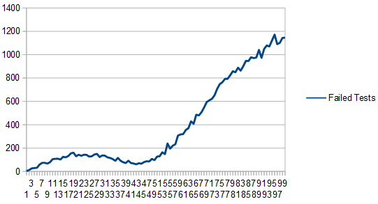
Here is the graph of the failure counts:

Here the box has a height of 2.8. It still works, but uses 2.8 samples on average which is less efficient:

Here’s the graph of failure counts:
Something interesting about this technique is that technically, the distribution you are sampling from doesn’t even have to be a PDF! If you have negative parts of the graph, they will be treated as zero, assuming your box has a minimum y of 0. Also, the fact that your function may not integrate to (have an area of) 1 doesn’t matter at all.
Here we take the PDF from the last examples, and take off the division by a constant, so that it doesn’t integrate to 1:

The interesting thing is that we get as output a normalized PDF (the red line), even though the distribution we were using to sample was not normalized (the blue line, which is mostly hidden behind the yellow line).
Here are the rejection counts:

Generating One PDF from Another PDF
In the last section we showed how to enclose a PDF in a box, make uniformly random 2d points, and use them to generate points from the PDF.
By enclosing it in a box, all we were really doing is putting it under a uniform distribition that was scaled up to be larger than the PDF at all points.
Now here’s the interesting thing: We aren’t limited to using the uniform distribution!
To generalize this technique, if you are trying to sample from a PDF 


Using this more generalized technique has one or two more steps than the other way, but allows for a tighter fit of a generating function, resulting in fewer samples thrown away.
Here’s how to do it:
- Generate a random number from the distribution g, and call it x.
- Calculate the percentage chance of x being chosen by getting a ratio of how likely that number is to be chosen in each PDF:
- Generate a uniform random number from 0 to 1. If it’s less than the value you just calculated, accept x as the random number, else reject it and go back to 1.

Let’s see this in action!
We’ll generate numbers in a Gaussian distribution with a mean of 15 and a standard deviation of 5. We’ll truncate it to +/- 3 standard deviations so we want to generate random numbers from [0,30).
To generate these numbers, we’ll draw random numbers from the PDF 
Here is how it looks doing this with 20,000 samples:

We generate random numbers along the red line, multiply them by 3 to make them be the yellow line. Then, at whatever point we are at on the x axis, we divide the blue line value by the yellow line value and use that as an acceptance probability. Doing this and counting numbers in a histogram gives us our result – the green line. Since the end goal is the blue line, you can see it is indeed working! With a larger number of samples, the green line would more closely match the blue line.
Here’s the graph of the failed tests:
We have to take on average 3 samples before we get a valid random number. That shouldn’t be too surprising because both PDF’s start with area of 1, but we are multiplying one of them by 3 to make it always be larger than the other.
Something else interesting you might notice is that we have a lot fewer failed tests where the two PDF functions are more similar.
That is the power of this technique: If you can cheaply and easily generate samples that are “pretty close” to a harder distribution to sample from, you can use this technique to more cheaply sample from it.
Something to note is that just like in the last section, the target PDF doesn’t necessarily need to be a real PDF with only positive values and integrating to 1. It would work just the same with a non PDF function, just so long as the PDF generating the random numbers you start with is always above the function.
Some Other Notes
There is family of techniques called “adaptive rejection sampling” that will change the PDF they are drawing from whenever there is a failed test.
Basically, if you imagine the PDF you are drawing from as being a bunch of line segments connected together, you could imagine that whenever you failed a test, you moved a line segment down to be closer to the curve, so that when you sampled from that area again, the chances would be lower that you’d fail the test again.
Taking this to the limit, your sampling PDF will eventually become the PDF you are trying to sample from, and then using this PDF will be a no-op.
These techniques are a continued area of research.
Something else to note is that rejection sampling can be used to find random points within shapes.
For instance, a random point on a triangle, ellipse or circle could be done by putting a (tight) bounding box around the shape, generating points randomly in that box, and only accepting ones within the inner shape.
This can be extended to 3d shapes as well.
Some shapes have better ways to generate points within them that don’t involve iteration and rejected samples, but if all else fails, rejection sampling does indeed work!
At some point in the future I’d like to look into “Markov Chain Monte Carlo” more deeply. It seems like a very interesting technique to approach this same problem, but I have no idea if it’s used often in graphics, especially real time graphics.
Code
Here is the code that generated all the data from this post. The data was visualized with open office.
#define _CRT_SECURE_NO_WARNINGS

#include <stdio.h>
#include <random>
#include <array>
#include <unordered_map>

template <size_t NUM_TEST_SAMPLES, size_t SIMULATED_DICE_SIDES, size_t ACTUAL_DICE_SIDES>
void TestDice (const char* fileName)
{
    // seed the random number generator
    std::random_device rd;
    std::mt19937 rng(rd());
    std::uniform_int_distribution<size_t> dist(0, ACTUAL_DICE_SIDES-1);

    // generate the histogram
    std::array<size_t, SIMULATED_DICE_SIDES> histogram = { 0 };
    size_t rejectedSamples = 0;
    for (size_t i = 0; i < NUM_TEST_SAMPLES; ++i)
    {
        size_t roll = dist(rng);
        while (roll >= SIMULATED_DICE_SIDES)
        {
            ++rejectedSamples;
            roll = dist(rng);
        }
        histogram[roll]++;
    }

    // write the histogram and rejected sample count to a csv
    // an extra 0 data point forces the graph to include 0 in the scale. hack to make the data not look noisier than it really is.
    FILE *file = fopen(fileName, "w+t");
    fprintf(file, "Actual Count, Expected Count, , %0.2f samples needed per roll on average.\n", (float(NUM_TEST_SAMPLES) + float(rejectedSamples)) / float(NUM_TEST_SAMPLES));
    for (size_t value : histogram)
        fprintf(file, "%zu,%zu,0\n", value, (size_t)(float(NUM_TEST_SAMPLES) / float(SIMULATED_DICE_SIDES)));
    fclose(file);
}

template <size_t NUM_TEST_SAMPLES, size_t NUM_HISTOGRAM_BUCKETS, typename PDF_LAMBDA>
void Test (const char* fileName, float maxPDFValue, const PDF_LAMBDA& PDF)
{
    // seed the random number generator
    std::random_device rd;
    std::mt19937 rng(rd());
    std::uniform_real_distribution<float> dist(0.0f, 1.0f);

    // generate the histogram
    std::array<size_t, NUM_HISTOGRAM_BUCKETS> histogram = { 0 };
    std::array<size_t, NUM_HISTOGRAM_BUCKETS> failedTestCounts = { 0 };
    size_t rejectedSamples = 0;
    for (size_t i = 0; i < NUM_TEST_SAMPLES; ++i)
    {
        // Generate a sample from the PDF by generating a random 2d point.
        // If the y axis of the value is <= the value returned by PDF(x), accept it, else reject it.
        // NOTE: this takes an unknown number of iterations, and technically may NEVER finish.
        float pointX = 0.0f;
        float pointY = 0.0f;
        bool validPoint = false;
        while (!validPoint)
        {
            pointX = dist(rng);
            pointY = dist(rng) * maxPDFValue;
            float pdfValue = PDF(pointX);
            validPoint = (pointY <= pdfValue);

            // track number of failed tests per histogram bucket
            if (!validPoint)
            {
                size_t bin = (size_t)std::floor(pointX * float(NUM_HISTOGRAM_BUCKETS));
                failedTestCounts[std::min(bin, NUM_HISTOGRAM_BUCKETS - 1)]++;
                ++rejectedSamples;
            }
        }

        // increment the correct bin in the histogram
        size_t bin = (size_t)std::floor(pointX * float(NUM_HISTOGRAM_BUCKETS));
        histogram[std::min(bin, NUM_HISTOGRAM_BUCKETS -1)]++;
    }

    // write the histogram and pdf sample to a csv
    FILE *file = fopen(fileName, "w+t");
    fprintf(file, "PDF, Simulated PDF, Generating Function, Failed Tests, %0.2f samples needed per value on average.\n", (float(NUM_TEST_SAMPLES) + float(rejectedSamples)) / float(NUM_TEST_SAMPLES));
    for (size_t i = 0; i < NUM_HISTOGRAM_BUCKETS; ++i)
    {
        float x = (float(i) + 0.5f) / float(NUM_HISTOGRAM_BUCKETS);
        float pdfSample = PDF(x);
        fprintf(file, "%f,%f,%f,%f\n",
            pdfSample,
            NUM_HISTOGRAM_BUCKETS * float(histogram[i]) / float(NUM_TEST_SAMPLES),
            maxPDFValue,
            float(failedTestCounts[i])
        );
    }
    fclose(file);
}

template <size_t NUM_TEST_SAMPLES, size_t NUM_HISTOGRAM_BUCKETS, typename PDF_LAMBDA>
void TestNotPDF (const char* fileName, float maxPDFValue, float normalizationConstant, const PDF_LAMBDA& PDF)
{
    // seed the random number generator
    std::random_device rd;
    std::mt19937 rng(rd());
    std::uniform_real_distribution<float> dist(0.0f, 1.0f);

    // generate the histogram
    std::array<size_t, NUM_HISTOGRAM_BUCKETS> histogram = { 0 };
    std::array<size_t, NUM_HISTOGRAM_BUCKETS> failedTestCounts = { 0 };
    size_t rejectedSamples = 0;
    for (size_t i = 0; i < NUM_TEST_SAMPLES; ++i)
    {
        // Generate a sample from the PDF by generating a random 2d point.
        // If the y axis of the value is <= the value returned by PDF(x), accept it, else reject it.
        // NOTE: this takes an unknown number of iterations, and technically may NEVER finish.
        float pointX = 0.0f;
        float pointY = 0.0f;
        bool validPoint = false;
        while (!validPoint)
        {
            pointX = dist(rng);
            pointY = dist(rng) * maxPDFValue;
            float pdfValue = PDF(pointX);
            validPoint = (pointY <= pdfValue);

            // track number of failed tests per histogram bucket
            if (!validPoint)
            {
                size_t bin = (size_t)std::floor(pointX * float(NUM_HISTOGRAM_BUCKETS));
                failedTestCounts[std::min(bin, NUM_HISTOGRAM_BUCKETS - 1)]++;
                ++rejectedSamples;
            }
        }

        // increment the correct bin in the histogram
        size_t bin = (size_t)std::floor(pointX * float(NUM_HISTOGRAM_BUCKETS));
        histogram[std::min(bin, NUM_HISTOGRAM_BUCKETS -1)]++;
    }

    // write the histogram and pdf sample to a csv
    FILE *file = fopen(fileName, "w+t");
    fprintf(file, "Function, Simulated PDF, Scaled Simulated PDF, Generating Function, Failed Tests, %0.2f samples needed per value on average.\n", (float(NUM_TEST_SAMPLES) + float(rejectedSamples)) / float(NUM_TEST_SAMPLES));
    for (size_t i = 0; i < NUM_HISTOGRAM_BUCKETS; ++i)
    {
        float x = (float(i) + 0.5f) / float(NUM_HISTOGRAM_BUCKETS);
        float pdfSample = PDF(x);
        fprintf(file, "%f,%f,%f,%f,%f\n",
            pdfSample,
            NUM_HISTOGRAM_BUCKETS * float(histogram[i]) / float(NUM_TEST_SAMPLES),
            NUM_HISTOGRAM_BUCKETS * float(histogram[i]) / float(NUM_TEST_SAMPLES) * normalizationConstant,
            maxPDFValue,
            float(failedTestCounts[i])
        );
    }
    fclose(file);
}

template <size_t NUM_TEST_SAMPLES, size_t NUM_HISTOGRAM_BUCKETS, typename PDF_F_LAMBDA, typename PDF_G_LAMBDA, typename INVERSE_CDF_G_LAMBDA>
void TestPDFToPDF (const char* fileName, const PDF_F_LAMBDA& PDF_F, const PDF_G_LAMBDA& PDF_G, float M, const INVERSE_CDF_G_LAMBDA& Inverse_CDF_G, float rngRange)
{
    // We generate a sample from PDF F by generating a sample from PDF G, and accepting it with probability PDF_F(x)/(M*PDF_G(x))

    // seed the random number generator
    std::random_device rd;
    std::mt19937 rng(rd());
    std::uniform_real_distribution<float> dist(0.0f, 1.0f);

    // generate the histogram
    std::array<size_t, NUM_HISTOGRAM_BUCKETS> histogram = { 0 };
    std::array<size_t, NUM_HISTOGRAM_BUCKETS> failedTestCounts = { 0 };
    size_t rejectedSamples = 0;
    for (size_t i = 0; i < NUM_TEST_SAMPLES; ++i)
    {
        // generate random points until we have one that's accepted
        // NOTE: this takes an unknown number of iterations, and technically may NEVER finish.
        float sampleG = 0.0f;
        bool validPoint = false;
        while (!validPoint)
        {
            // Generate a sample from the soure PDF G
            sampleG = Inverse_CDF_G(dist(rng));

            // calculate the ratio of how likely we are to accept this sample
            float acceptChance = PDF_F(sampleG) / (M * PDF_G(sampleG));

            // see if we should accept it
            validPoint = dist(rng) <= acceptChance;

            // track number of failed tests per histogram bucket
            if (!validPoint)
            {
                size_t bin = (size_t)std::floor(sampleG * float(NUM_HISTOGRAM_BUCKETS) / rngRange);
                failedTestCounts[std::min(bin, NUM_HISTOGRAM_BUCKETS - 1)]++;
                ++rejectedSamples;
            }
        }

        // increment the correct bin in the histogram
        size_t bin = (size_t)std::floor(sampleG * float(NUM_HISTOGRAM_BUCKETS) / rngRange);
        histogram[std::min(bin, NUM_HISTOGRAM_BUCKETS - 1)]++;
    }

    // write the histogram and pdf sample to a csv
    FILE *file = fopen(fileName, "w+t");
    fprintf(file, "PDF F,PDF G,Scaled PDF G,Simulated PDF,Failed Tests,%0.2f samples needed per value on average.\n", (float(NUM_TEST_SAMPLES) + float(rejectedSamples)) / float(NUM_TEST_SAMPLES));
    for (size_t i = 0; i < NUM_HISTOGRAM_BUCKETS; ++i)
    {
        float x = (float(i) + 0.5f) * rngRange / float(NUM_HISTOGRAM_BUCKETS);

        fprintf(file, "%f,%f,%f,%f,%f\n",
            PDF_F(x),
            PDF_G(x),
            PDF_G(x)*M,
            NUM_HISTOGRAM_BUCKETS * float(histogram[i]) / (float(NUM_TEST_SAMPLES)*rngRange),
            float(failedTestCounts[i])
        );
    }
    fclose(file);
}

int main(int argc, char **argv)
{
    // Dice
    {
        // Simulate a 5 sided dice with a 6 sided dice
        TestDice<10000, 5, 6>("test1_5_6.csv");

        // Simulate a 5 sided dice with a 20 sided dice
        TestDice<10000, 5, 20>("test1_5_20.csv");
    }

    // PDF y=2x, simulated with a uniform distribution
    {
        auto PDF = [](float x) { return 2.0f * x; };

        Test<1000, 100>("test2_1k.csv", 2.0f, PDF);
        Test<100000, 100>("test2_100k.csv", 2.0f, PDF);
        Test<1000000, 100>("test2_1m.csv", 2.0f, PDF);
    }

    // PDF y=(x^3-10x^2+5x+11)/10.417, simulated with a uniform distribution
    {
        auto PDF = [](float x) {return (x*x*x - 10.0f*x*x + 5.0f*x + 11.0f) / (10.417f); };
        Test<10000000, 100>("test3_10m_1_15.csv", 1.15f, PDF);
        Test<10000000, 100>("test3_10m_1_5.csv", 1.5f, PDF);
        Test<10000000, 100>("test3_10m_2_8.csv", 2.8f, PDF);
    }

    // function (not PDF, Doesn't integrate to 1!) y=(x^3-10x^2+5x+11), simulated with a scaled up uniform distribution
    {
        auto PDF = [](float x) {return (x*x*x - 10.0f*x*x + 5.0f*x + 11.0f); };
        TestNotPDF<10000000, 100>("test4_10m_12_5.csv", 12.5f, 10.417f, PDF);
    }

    // Generate samples from PDF F using samples from PDF G.  random numbers are from 0 to 30.
    // F PDF = gaussian distribution, mean 15, std dev of 5.  Truncated to +/- 3 stddeviations.
    // G PDF = x*0.002222
    // G CDF = 0.001111 * x^2
    // G inverted CDF = (1000 * sqrt(x)) / sqrt(1111)
    // M = 3
    {
        // gaussian PDF F
        const float mean = 15.0f;
        const float stddev = 5.0f;
        auto PDF_F = [=] (float x) -> float
        {
            return (1.0f / (stddev * sqrt(2.0f * (float)std::_Pi))) * std::exp(-0.5f * pow((x - mean) / stddev, 2.0f));
        };

        // PDF G
        auto PDF_G = [](float x) -> float
        {
            return x * 0.002222f;
        };

        // Inverse CDF of G
        auto Inverse_CDF_G = [] (float x) -> float
        {
            return 1000.0f * std::sqrtf(x) / std::sqrtf(1111.0f);
        };

        TestPDFToPDF<20000, 100>("test5.csv", PDF_F, PDF_G, 3.0f, Inverse_CDF_G, 30.0f);
    }

    return 0;
}


 where
where ![x \in [0,1]](https://s0.wp.com/latex.php?latex=x+%5Cin+%5B0%2C1%5D&bg=ffffff&fg=666666&s=0&c=20201002) . The graph looks like this:
. The graph looks like this:
 where
where 


 which looks like this:
 and looks like this:


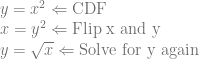
 . The area under that curve where x is in [0,1) is 1.0 and it’s non negative everywhere in that range too, so it’s a valid PDF.
 for the CDF. Then we invert the CDF:
![y=x^3 \Leftarrow \text{CDF}\\ x=y^3 \Leftarrow \text{Flip x and y}\\ y=\sqrt[3]{x} \Leftarrow \text{Solve for y again}](https://s0.wp.com/latex.php?latex=y%3Dx%5E3+%5CLeftarrow+%5Ctext%7BCDF%7D%5C%5C+x%3Dy%5E3+%5CLeftarrow+%5Ctext%7BFlip+x+and+y%7D%5C%5C+y%3D%5Csqrt%5B3%5D%7Bx%7D+%5CLeftarrow+%5Ctext%7BSolve+for+y+again%7D&bg=ffffff&fg=666666&s=0&c=20201002)


