This Post In Short:
- Fit a curve of degree N to a data set, getting data points 1 at a time.
- Storage Required: 3*N+2 values.
- Update Complexity: roughly 3*N+2 additions and multiplies.
- Finalize Complexity: Solving Ax=b where A is an (N+1)x(N+1) matrix and b is a known vector. (Sample code inverts A matrix and multiplies by b, Gaussian elimination is better though).
- Simple C++ code and HTML5 demo at bottom!
I was recently reading a post from a buddy on OIT or “Order Independent Transparency” which is an open problem in graphics:
Fourier series based OIT and why it won’t work
In the article he talks about trying to approximate a function per pixel and shows the details of some methods he tried. One of the difficulties with the problem is that during a render you can get any number of triangles affecting a specific pixel, but you need a fixed and bounded size amount of storage per pixel for those variable numbers of data points.
That made me wonder: Is there an algorithm that can approximate a data set with a function, getting only one data point at a time, and end up with a decent approximation?
It turns out that there is one, at least one that I am happy with: Incremental Least Squares Curve Fitting.
While this perhaps doesn’t address all the problems that need addressing for OIT specifically, I think this is a great technique for programming in general, and I’m betting it still has it’s uses in graphics, for other times when you want to approximate a data set per pixel.
We’ll work through a math oriented way to do it, and then we’ll convert it into an equivalent and simpler programmer friendly version.
At the bottom of the post is some simple C++ that implements everything we talk about and the image below is a screenshot of an an interactive HTML5 demo I made: Least Squares Curve Fitting

Mathy Version
I found out about this technique by asking on math stack exchange and got a great (if not mathematically dense!) answer:
Math Stack Exchange: Creating a function incrementally

I have to admit, I’m not so great with matrices outside of the typical graphics/gamedev usage cases of transormation and related, so it took me a few days to work through it and understand it all. If reading that answer made your eyes go blurry, give my explanation a shot. I’m hoping I gave step by step details enough such that you too can understand what the heck he was talking about. If not, let me know where you got lost and I can explain better and update the post.
The first thing we need to do is figure out what degree of a function we want to approximate our data with. For our example we’ll pick a degree 2 function, also known as a quadratic function. That means that when we are done we will get out a function of the form below:

We will give data points to the equation and it will calculate the values of a,b and c that approximate our function by minimizing the sum of the squared distance from each point to the curve.
We’ll deal with regular least squared fitting before moving onto incremental, so here’s the data set we’ll be fitting our quadratic curve to:

The x values in my data set start at 1 and count up by 1, but that is not a requirement. You can use whatever x and y values you want to fit a curve to.
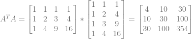
Next we need to calculate the matrix 


When we plug in our specific x values we get this:

Calculating it out we get this:

Next we need to calculate the matrix 
Next we need to find the inverse of that matrix to get 

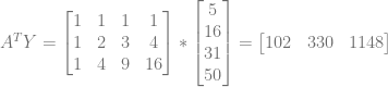
The next thing we need to calculate is 
And finally, to calculate the coefficients of our quadratic function, we need to calculate 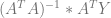

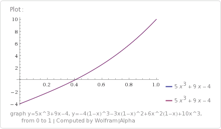
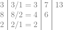
Those coefficients are listed in power order of x, so the first value -2 is the coefficient for x^0, 5 is the coefficient for x^1 and 2 is the coefficient for x^2. That gives us the equation:

If you plug in the x values from our data set, you’ll find that this curve perfectly fits all 4 data points.
It won’t always be (and usually won’t be) that a resulting curve matches the input set for all values. It just so happened that this time it does. The only guarantee you’ll get when fitting a curve to the data points is that the squared distance of the point to the curve (distance on the Y axis only, so vertical distance), is minimized for all data points.
Now that we’ve worked through the math, let’s make some observations and make it more programmer friendly.
Making it Programmer Friendly
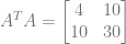
Let’s look at the

One thing you probably noticed right away is that it’s symmetric across the diagonal. Another thing you may have noticed is that there are only 5 unique values in that matrix.
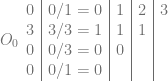
As it turns out, those 5 values are just the sum of the x values, when those x values are raised to increasing powers.
- If you take all x values of our data set, raise them to the 0th power and sum the results, you get 4.
- If you take all x values of our data set, raise them to the 1st power and sum the results, you get 10.
- If you take all x values of our data set, raise them to the 2nd power and sum the results, you get 30.
- If you take all x values of our data set, raise them to the 3rd power and sum the results, you get 100.
- If you take all x values of our data set, raise them to the 4th power and sum the results, you get 354.
Further more, the power of the x values in each part of the matrix is the zero based x axis index plus the zero based y axis index. Check out what i mean below, which shows which power the x values are taken to before being summed for each location in the matrix:

That is interesting for two reasons…
- This tells us that we only really need to store the 5 unique values, and that we can reconstruct the full matrix later when it’s time to calculate the coefficients.
- It also tells us that if we’ve fit a curve to some data points, but then want to add a new data point, that we can just raise the x value of our new data point to the different powers and add it into these 5 values we already have stored. In other words, the
This generalizes beyond quadratic functions too luckily. If you are fitting your data points with a degree N curve, the
As a concrete example, a cubic fit will have an
So, the
That is great, but there is another value we need to look at too, which is the

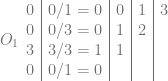
There are some patterns to this vector too luckily. You may have noticed that the first entry is the sum of the Y values from our data set. It’s actually the sum of the y values multiplied by the x values raised to the 0th power.
The next number is the sum of the y values multiplied by the x values raised to the 1st power, and so on.
To generalize it, each entry in that vector is the sum of taking the x from each data point, raising it to the power that is the index in the vector, and multiplying it by the y value.
- Taking each data point’s x value, raising it to the 0th power, multiplying by the y value, and summing the results gives you 102.
- Taking each data point’s x value, raising it to the 1st power, multiplying by the y value, and summing the results gives you 330.
- Taking each data point’s x value, raising it to the 2nd power, multiplying by the y value, and summing the results gives you 1148.
So, this vector is incrementally updatable too. When you get a new data point, for each entry in the vector, you take the x value to the specific power, multiply by y, and add that result to the entry in the vector.
This generalizes for other curve types as well. If you are fitting your data points with a degree N curve, the
As a concrete example, a cubic fit will have an
Combining the storage needs of the values needed for the
Algorithm Summarized
Here is a summary of the algorithm:
- First decide on the degree of the fit you want. Call it N.
- Ensure you have storage space for 3*N+2 values and initialize them all to zero. These represent the (N+1)*2-1 values needed for the
- For each data point you get, you will need to update both the
- for(i in ATA) ATA[i] += x^i
- for(i in ATY) ATY[i] += x^i*y
- When it’s time to calculate the coefficients of your polynomial, convert the ATA values back into the
Pretty simple right?
Not Having Enough Points
When working through the mathier version of this algorithm, you may have noticed that if we were trying to fit using a degree N curve, that we needed N+1 data points at minimum for the math to even be able to happen.
So, you might ask, what happens in the real world, such as in a pixel shader, where we decide to do a cubic fit, but end up only getting 1 data point, instead of the 4 minimum that we need?
Well, first off, if you use the programmer friendly method of incrementally updating ATA and ATY, you’ll end up with an uninvertible matrix (0 determinant), but that doesn’t really help us any besides telling us when we don’t have enough data.
There is something pretty awesome hiding here though. Let’s look at the ATA matrix and ATY values from our quadratic example again.


The above values are for a quadratic fit. What if we wanted a linear fit instead? Well… the upper left 2×2 matrix in ATA is the ATA matrix for the linear fit! Also, the first two values in the ATY vector is the ATY vector if we were doing a linear fit.

You can verify that the linear fit above is correct if you want, but let’s take it down another degree, down to approximating the fit with a point. They become scalars instead of matrices and vectors:

If we take the inverse of ATA and multiply it by ATY, we get:
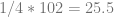
if you average the Y values of our input data, you’ll find that it is indeed 25.5, so we have verified that it does give us a degree 0 fit.
This is neat and all, but how can we KNOW if we’ve collected enough data or not? Do we just try to invert our ATA matrix, and if it fails, try one degree lower, repeatedly, until we succeed or fail at a degree 0 approximation? Do we maybe instead store a counter to keep track of how many points we have seen?
Luckily no, and maybe you have already put it together. The first value in the ATA array actually TELLS you how many points you have been given. You can use that to decide what degree you are going to have to actually fit the data set to when it’s time to calculate your coefficients, to avoid the uninvertible matrix and still get your data fit.
Interesting Tid Bits
Something pretty awesome about this algorithm is that it can work in a multithreaded fashion very easily. One way would be to break apart the work into multiple job threads, have them calculate ATA and ATY independently, and then sum them all together on the main thread. Another way to do it would be to let all threads share the same ATA and ATY storage, but to use an atomic add operation to update them.
Going the atomic add route, I think this could be a relatively GPU friendly algorithm. You could use actual atomic operations in your shader code, or you could use alpha blending to add your result in.
Even though we saw it in the last section, I’ll mention it again. If you do a degree 0 curve fit to data points (aka fitting a point to the data), this algorithm is mathematically equivalent to just taking the average y value. The ATA values will have a single value which is the sum of the x values to the 0th degree, so will be the count of how many x items there are. The ATY values will also have only a single value, which will be the sum of the x^0*y values, so will be the sum of the y values. Taking the inverse of our 1×1 ATA matrix will give us one divided by how many items there are, so when we multiply that by the ATA vector which only has one item, it will be the same as if we divided our Y value sum by how many data points we had. So, in a way, this algorithm seems to be some sort of generalization of averaging, which is weird to me.
Another cool thing: if you have the minimum number of data points for your degree (aka degree+1 data points) or fewer, you can actually use the ATA and ATY values to get back your ORIGINAL data points – both the X and the Y values! I’ll leave it as an exercise for you, but if you look at it, you will always have more equations than you do unknowns.
If reconstructing the original data points is important to you, you could also have this algorithm operate in two modes.
Basically, always use the ATA[0] storage space to count the number of data points you’ve been given, since that is it’s entire purpose. You can then use the rest of the storage space as RAW data storage for your 2d input values. As soon as adding another value would cause you to overflow your storage, you could process your data points into the correct format of storing just ATA and ATY values, so that from then on, it was an approximation, instead of explicit point storage.
When decoding those values, you would use the ATA[0] storage space to know whether the rest of the storage contained ATA and ATY values, or if they contained data points. If they contained data points, you would also know how many there were, and where they were in the storage space, using the same logic to read data points out as you used to put them back in – basically like saying that the first data point goes immediately after ATA[0], the second data point after that, etc.
The last neat thing, let’s say that you are in a pixel shader as an exmaple, and that you wanted to approximate 2 different values for each pixel, but let’s say that the X value was always the same for these data sets – maybe you are approximating two different values over depth of the pixel for instance so X of both data points is the depth, but the Y values of the data points are different.
If you find yourself in a situation like this, you don’t actually need to pay the full cost of storage to have a second approximation curve.
Since the ATA values are all based on powers of the x values only, the ATA values would be the same for both of these data sets. You only need to pay the cost of the ATY values for the second curve.
This means that fitting a curve costs an initial 3*degree+2 in storage, but each additional curve only costs degree+1 in storage.
Also, since the ATA storage for a curve of degree N also contains the same values used for a curve of degree N-1, N-2, etc, you don’t have to use the same degree when approximating multiple values using the same storage. Your ATA just has to be large enough to hold the largest degree curve, and then you can have ATY values that are sized to the degree of the curve you want to use to approximate each data set.
This way, if you have limited storage, you could perhaps cubically fit one data set, and then linearly fit another data set where accuracy isn’t as important.
For that example, you would pay 11 values of storage for the cubic fit, and then only 2 more values of storage to have a linear fit of some other data.
Example Code
There is some example code below that implements the ideas from this post.
The code is meant to be clear and readable firstly, with being a reasonably decent implementation second. If you are using this in a place where you want high precision and/or high speeds, there are likely both macro and micro optimizations and code changes to be made. The biggest of these is probably how the matrix is inverted.
You can read more on the reddit discussion: Reddit: Incremental Least Squares Curve Fitting
Here’s a run of the example code:

Here is the example code:
#include <stdio.h>
#include <array>

//====================================================================
template<size_t N>
using TVector = std::array<float, N>;

template<size_t M, size_t N>
using TMatrix = std::array<TVector<N>, M>;

template<size_t N>
using TSquareMatrix = TMatrix<N,N>;

typedef TVector<2> TDataPoint;

//====================================================================
template <size_t N>
float DotProduct (const TVector<N>& A, const TVector<N>& B)
{
    float ret = 0.0f;
    for (size_t i = 0; i < N; ++i)
        ret += A[i] * B[i];
    return ret;
}

//====================================================================
template <size_t M, size_t N>
void TransposeMatrix (const TMatrix<M, N>& in, TMatrix<N, M>& result)
{
    for (size_t j = 0; j < M; ++j)
        for (size_t k = 0; k < N; ++k)
            result[k][j] = in[j][k];
}

//====================================================================
template <size_t M, size_t N>
void MinorMatrix (const TMatrix<M, N>& in, TMatrix<M-1, N-1>& out, size_t excludeI, size_t excludeJ)
{
    size_t destI = 0;
    for (size_t i = 0; i < N; ++i)
    {
        if (i != excludeI)
        {
            size_t destJ = 0;
            for (size_t j = 0; j < N; ++j)
            {
                if (j != excludeJ)
                {
                    out[destI][destJ] = in[i][j];
                    ++destJ;
                }
            }
            ++destI;
        }
    }
}

//====================================================================
template <size_t M, size_t N>
float Determinant (const TMatrix<M,N>& in)
{
    float determinant = 0.0f;
	TMatrix<M - 1, N - 1> minor;
    for (size_t j = 0; j < N; ++j)
    {
        MinorMatrix(in, minor, 0, j);

        float minorDeterminant = Determinant(minor);
        if (j % 2 == 1)
            minorDeterminant *= -1.0f;

        determinant += in[0][j] * minorDeterminant;
    }
    return determinant;
}

//====================================================================
template <>
float Determinant<1> (const TMatrix<1,1>& in)
{
	return in[0][0];
}

//====================================================================
template <size_t N>
bool InvertMatrix (const TSquareMatrix<N>& in, TSquareMatrix<N>& out)
{
    // calculate the cofactor matrix and determinant
    float determinant = 0.0f;
    TSquareMatrix<N> cofactors;
    TSquareMatrix<N-1> minor;
    for (size_t i = 0; i < N; ++i)
    {
        for (size_t j = 0; j < N; ++j)
        {
            MinorMatrix(in, minor, i, j);

            cofactors[i][j] = Determinant(minor);
            if ((i + j) % 2 == 1)
                cofactors[i][j] *= -1.0f;

            if (i == 0)
                determinant += in[i][j] * cofactors[i][j];
        }
    }

    // matrix cant be inverted if determinant is zero
    if (determinant == 0.0f)
        return false;

    // calculate the adjoint matrix into the out matrix
    TransposeMatrix(cofactors, out);

    // divide by determinant
    float oneOverDeterminant = 1.0f / determinant;
    for (size_t i = 0; i < N; ++i)
        for (size_t j = 0; j < N; ++j)
            out[i][j] *= oneOverDeterminant;
    return true;
}

//====================================================================
template <>
bool InvertMatrix<2> (const TSquareMatrix<2>& in, TSquareMatrix<2>& out)
{
    float determinant = Determinant(in);
    if (determinant == 0.0f)
        return false;

    float oneOverDeterminant = 1.0f / determinant;
    out[0][0] =  in[1][1] * oneOverDeterminant;
    out[0][1] = -in[0][1] * oneOverDeterminant;
    out[1][0] = -in[1][0] * oneOverDeterminant;
    out[1][1] =  in[0][0] * oneOverDeterminant;
    return true;
}

//====================================================================
template <size_t DEGREE>  // 1 = linear, 2 = quadratic, etc
class COnlineLeastSquaresFitter
{
public:
    COnlineLeastSquaresFitter ()
    {
        // initialize our sums to zero
        std::fill(m_SummedPowersX.begin(), m_SummedPowersX.end(), 0.0f);
        std::fill(m_SummedPowersXTimesY.begin(), m_SummedPowersXTimesY.end(), 0.0f);
    }

    void AddDataPoint (const TDataPoint& dataPoint)
    {
        // add the summed powers of the x value
        float xpow = 1.0f;
        for (size_t i = 0; i < m_SummedPowersX.size(); ++i)
        {
            m_SummedPowersX[i] += xpow;
            xpow *= dataPoint[0];
        }

        // add the summed powers of the x value, multiplied by the y value
        xpow = 1.0f;
        for (size_t i = 0; i < m_SummedPowersXTimesY.size(); ++i)
        {
            m_SummedPowersXTimesY[i] += xpow * dataPoint[1];
            xpow *= dataPoint[0];
        }
    }

    bool CalculateCoefficients (TVector<DEGREE+1>& coefficients) const
    {
        // initialize all coefficients to zero
        std::fill(coefficients.begin(), coefficients.end(), 0.0f);

        // calculate the coefficients
        return CalculateCoefficientsInternal<DEGREE>(coefficients);
    }

private:

    template <size_t EFFECTIVEDEGREE>
    bool CalculateCoefficientsInternal (TVector<DEGREE + 1>& coefficients) const
    {
        // if we don't have enough data points for this degree, try one degree less
        if (m_SummedPowersX[0] <= EFFECTIVEDEGREE)
            return CalculateCoefficientsInternal<EFFECTIVEDEGREE - 1>(coefficients);

        // Make the ATA matrix
        TMatrix<EFFECTIVEDEGREE + 1, EFFECTIVEDEGREE + 1> ATA;
        for (size_t i = 0; i < EFFECTIVEDEGREE + 1; ++i)
            for (size_t j = 0; j < EFFECTIVEDEGREE + 1; ++j)
                ATA[i][j] = m_SummedPowersX[i + j];

        // calculate inverse of ATA matrix
        TMatrix<EFFECTIVEDEGREE + 1, EFFECTIVEDEGREE + 1> ATAInverse;
        if (!InvertMatrix(ATA, ATAInverse))
            return false;

        // calculate the coefficients for this degree. The higher ones are already zeroed out.
        TVector<EFFECTIVEDEGREE + 1> summedPowersXTimesY;
        std::copy(m_SummedPowersXTimesY.begin(), m_SummedPowersXTimesY.begin() + EFFECTIVEDEGREE + 1, summedPowersXTimesY.begin());
        for (size_t i = 0; i < EFFECTIVEDEGREE + 1; ++i)
            coefficients[i] = DotProduct(ATAInverse[i], summedPowersXTimesY);
        return true;
    }

    // Base case when no points are given, or if you are fitting a degree 0 curve to the data set.
    template <>
    bool CalculateCoefficientsInternal<0> (TVector<DEGREE + 1>& coefficients) const
    {
        if (m_SummedPowersX[0] > 0.0f)
            coefficients[0] = m_SummedPowersXTimesY[0] / m_SummedPowersX[0];
        return true;
    }

    // Total storage space (# of floats) needed is 3 * DEGREE + 2
    // Where y is number of values that need to be stored and x is the degree of the polynomial
    TVector<(DEGREE + 1) * 2 - 1>   m_SummedPowersX;
    TVector<DEGREE + 1>             m_SummedPowersXTimesY;
};

//====================================================================
template <size_t DEGREE>
void DoTest(const std::initializer_list<TDataPoint>& data)
{
	printf("Fitting a curve of degree %zi to %zi data points:n", DEGREE, data.size());

    COnlineLeastSquaresFitter<DEGREE> fitter;

	// show data
    for (const TDataPoint& dataPoint : data)
		printf("  (%0.2f, %0.2f)n", dataPoint[0], dataPoint[1]);

	// fit data
    for (const TDataPoint& dataPoint : data)
        fitter.AddDataPoint(dataPoint);

	// calculate coefficients if we can
	TVector<DEGREE+1> coefficients;
	bool success = fitter.CalculateCoefficients(coefficients);
	if (!success)
	{
		printf("ATA Matrix could not be inverted!n");
		return;
	}

	// print the polynomial
	bool firstTerm = true;
	printf("y = ");
    bool showedATerm = false;
	for (int i = (int)coefficients.size() - 1; i >= 0; --i)
	{
		// don't show zero terms
		if (std::abs(coefficients[i]) < 0.00001f)
			continue;

        showedATerm = true;

		// show an add or subtract between terms
		float coefficient = coefficients[i];
		if (firstTerm)
			firstTerm = false;
		else if (coefficient >= 0.0f)
			printf(" + ");
		else
		{
			coefficient *= -1.0f;
			printf(" - ");
		}

		printf("%0.2f", coefficient);

		if (i > 0)
			printf("x");

		if (i > 1)
			printf("^%i", i);
	}
    if (!showedATerm)
        printf("0");
	printf("nn");
}

//====================================================================
int main (int argc, char **argv)
{
	// Point - 1 data points
    DoTest<0>(
        {
            TDataPoint{ 1.0f, 2.0f },
        }
    );

	// Point - 2 data points
    DoTest<0>(
        {
            TDataPoint{ 1.0f, 2.0f },
            TDataPoint{ 2.0f, 4.0f },
        }
    );

	// Linear - 2 data points
    DoTest<1>(
        {
            TDataPoint{ 1.0f, 2.0f },
            TDataPoint{ 2.0f, 4.0f },
        }
    );

	// Linear - 3 colinear data points
    DoTest<1>(
        {
            TDataPoint{ 1.0f, 2.0f },
            TDataPoint{ 2.0f, 4.0f },
            TDataPoint{ 3.0f, 6.0f },
        }
    );

	// Linear - 3 non colinear data points
    DoTest<1>(
        {
            TDataPoint{ 1.0f, 2.0f },
            TDataPoint{ 2.0f, 4.0f },
            TDataPoint{ 3.0f, 5.0f },
        }
    );

	// Quadratic - 3 colinear data points
    DoTest<2>(
        {
            TDataPoint{ 1.0f, 2.0f },
            TDataPoint{ 2.0f, 4.0f },
            TDataPoint{ 3.0f, 6.0f },
        }
    );

	// Quadratic - 3 data points
    DoTest<2>(
        {
            TDataPoint{ 1.0f, 5.0f },
            TDataPoint{ 2.0f, 16.0f },
            TDataPoint{ 3.0f, 31.0f },
        }
    );

	// Cubic - 4 data points
    DoTest<3>(
        {
            TDataPoint{ 1.0f, 5.0f },
            TDataPoint{ 2.0f, 16.0f },
            TDataPoint{ 3.0f, 31.0f },
            TDataPoint{ 4.0f, 16.0f },
        }
    );

	// Cubic - 2 data points
    DoTest<3>(
        {
            TDataPoint{ 1.0f, 7.0f },
            TDataPoint{ 3.0f, 17.0f },
        }
    );

	// Cubic - 1 data point
    DoTest<3>(
        {
            TDataPoint{ 1.0f, 7.0f },
        }
    );

	// Cubic - 0 data points
    DoTest<3>(
        {
        }
    );

    system("pause");
    return 0;
}
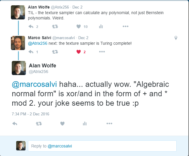
Feedback
There’s some interesting feedback on twitter.
Links
Here’s an interactive demo to let you get a feel for how least squares curve fitting behaves:
Least Squares Curve Fitting
Wolfram Mathworld: Least Squares Fitting
Wikipedia: Least Squares Fitting
Inverting a 2×2 Matrix
Inverting Larger Matrices
A good online polynomial curve fitting calculator
By the way, the term for an algorithm which works incrementally by taking only some of the data at a time is called an “online algorithm”. If you are ever in search of an online algorithm to do X (whatever X may be), using this term can be very helpful when searching for such an algorithm, or when asking people if such an algorithm exists (like on stack exchange). Unfortunately, online is a bit overloaded in the modern world, so it can also give false hits (;
Wikipedia: Online algorithm


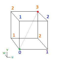
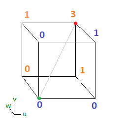
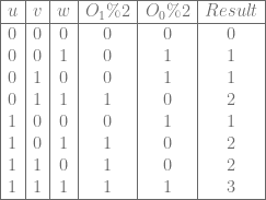
 will be the 1’s place output bit (least significant bit), and
  will be the 2’s place output bit (most significant bit). Our 3 input bits will be u,v,w.
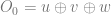

 ), and that XOR (
 ) is addition while AND is multiplication. This gives the formulas below:


 or
or  or by a constant or by another variable completely. My hope was that I’d be able to make the technique more generic and open it up to a larger family of equations, so people weren’t limited to just Bernstein polynomials.
 ) to “Bernstein Basis” (which looks like
  ) so long as they are the same degree.
 , that we can make this technique work for that too. The technique got a little closer to arbitrary equation evaluation. Neat!
 coefficient, then the
  coefficient and continuing on to the highest value
  :
:


 instead of
  and also setting
  .
.
 term, so it’s coefficient is 0.