Life update: I’m now doing applied graphics research at EA SEED and really digging it. Really great people, great work to be done, and lots of freedom to do it. I’m really stoked, to be honest.
In a previous post, I wrote about how to calculate the distance between two points in a rectangle, where the rectangle edges wrapped around. That is, if you leave the rectangle by going past the right edge, you’d end up coming out of the left edge. If you go past the top edge, you’d come out of the bottom edge.
This weird space can be thought of as a toroid, or a doughnut. If you start at a point on a doughnut and go “upwards” on the surface, you’ll circle around back to where you started. Similarly, going left, you’ll circle around the doughnut and come back to where you started. More technically, this space is a “flat toroid” though, so isn’t quite the same thing as a doughnut. Video games have used this space for their game worlds, such as the classic “Asteroids”.
Asteroids: One of the first of many games to take place on the surface of a doughnut
I was recently experimenting with something (the experiment failed unfortunately ☹️) that involved working in a disk where going to the edge of the disk would teleport you to the center of the disk, and going to the center of the disk would teleport you to the edge of the disk. It’s like if you squished a doughnut flat to make the center hole infinitely small, and you removed the back side of the doughnut.
As part of this work, I needed to be able to calculate the distance between two points in this strange space.
It was a fun problem, so maybe you want to give it a shot before i explain how I did it. I’d love to hear what you come up with, either here as a comment on this post, or on twitter at https://twitter.com/Atrix256.
My Solution
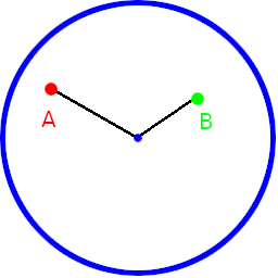
Ok so I knew that there would be a few ways to get from a point A to a point B in this toroidal disk, and that we’d want to take the shortest of these paths as the length between them.
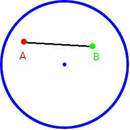
One path would be the line in the circle between the points.
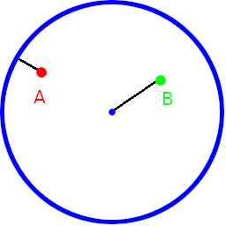
Another path would be from point A to the edge of the circle, to get to the center, and from the center to point B. It’s interesting to note that these lines don’t have to be parallel!
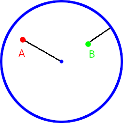
Another path would be from point A to the center of the circle to get to the edge, and from the edge to point B.
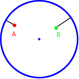
Now for some stranger cases…
You could go from point A to the edge, to the center of the circle, then back to the edge at a different location and to point B.
You could also go form point A to the center, change direction and go to point B. This last case could only be as short as the “interior” path at minimum, so isn’t really a case we have to consider, but I’m including it for completeness.
Ok so we could turn this into code with a bunch of if statements to handle each case, but we can simplify this logic quite a bit.
First up, we do have to calculate the distance between the points in the circle the normal way, there’s no avoiding that. We’ll call that the “interior distance”.
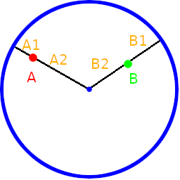
Next, think about the paths point A can take to point B that aren’t through the disk. It can either go to the edge or the center, and we’ll want to keep whichever is shorter as the distance for the first part of the “exterior distance”. Since we want to take the shortest path to the center or the edge, we can just use the point’s radius as the distance form the center and 1.0 – radius as the distance from the edge (assuming a radius 1 circle). We’ll take the minimum distance between those two as the first part of the exterior distance path.
Next, it doesn’t matter if point A went to the center or the edge, the path can come out of either the center or edge and continue to point B. So, we again want the minimum of the distances: point B to the edge of the disk, or point B to the center of the disk. once again it’s the minimum of the radius and 1.0 – radius.
Adding those two distances together we get the “exterior distance”
The “Exterior Distance” Is min(A1, A2) + min(B1, B2)
The final answer we return as the distance between point A and B is whichever is smaller: the interior or exterior distance.
A fun thing is that while we have been working in 2 dimensions, this actually works for any dimension.
Here is some C++ code to calculate the distance:
// walking past the end of the circle brings you back to the center, and vice versa
// Assumes your points are in [0,1)^N with a disk center of (0.5, 0.5, ...)
template <size_t N>
float DistanceUnitDiskTorroidal(const std::array<float, N>& v1, const std::array<float, N>& v2)
{
    // Calculate the distance between the points going through the disk.
    // This is the "internal" distance.
    float distanceInternal = Distance(v1, v2);

    // The external distance is the distance between the points if going through the center
    // or past the edges.
    // This is the sum of the distance between each point and either the circle edge or the
    // circle center, whichever is closer.
    float distanceExternal1 = Length(v1 - 0.5f);
    distanceExternal1 = std::min(distanceExternal1, 0.5f - distanceExternal1);

    float distanceExternal2 = Length(v2 - 0.5f);
    distanceExternal2 = std::min(distanceExternal2, 0.5f - distanceExternal2);

    float distanceExternal = distanceExternal1 + distanceExternal2;

    // return whichever is less, between the internal and external distance.
    return std::min(distanceInternal, distanceExternal);
}
Again, I’d love to hear your thoughts, or any alternative methods you may have come up with, either here or on twitter at https://twitter.com/Atrix256. Thanks for reading!
Update
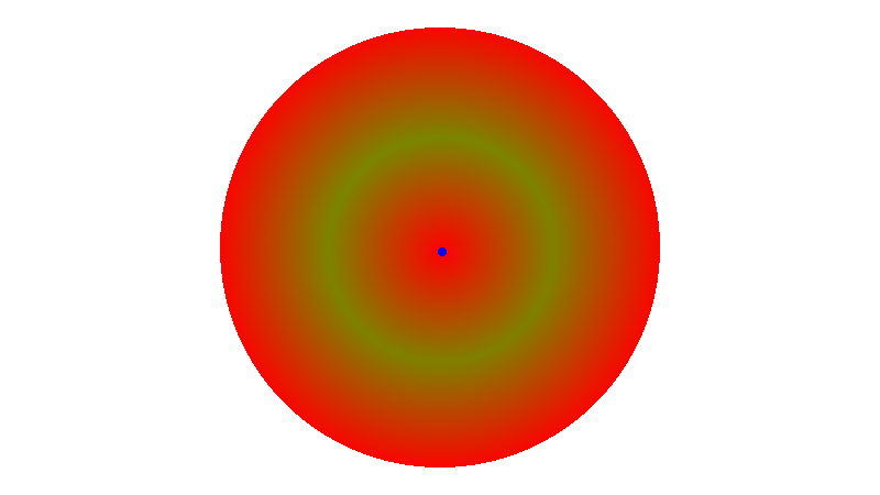
On twitter, https://twitter.com/Mal_loc mentioned that it would be nice to see the distance from one point to the rest of them visualized, to get a better sense of how this distance function worked. That was a great idea so i made an interactive shadertoy: https://www.shadertoy.com/view/NsBcDD
Here are a few images. The blue dot is the point that the distances are calculated from. Red is no distance, Green is full distance.
In 2014, Jorge Jimenez from Activision presented a type of noise optimized for use with Temporal Anti Aliasing called Interleaved Gradient Noise or IGN (http://www.iryoku.com/next-generation-post-processing-in-call-of-duty-advanced-warfare). This noise helps the neighborhood sampling history rejection part of TAA be more accurate, allowing the render to be closer to ground truth. IGN was ahead of it’s time. It still isn’t as well known or understood as it should be, and it shows the way for further advancements.
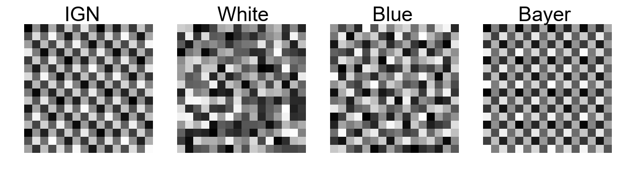
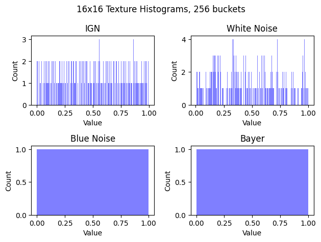
IGN can be used whenever you need a per pixel random number in rendering, and in this post we’ll compare and contrast IGN against three of its cousins: white noise, blue noise and Bayer matrices. Below are the 16×16 textures that we’ll be using for comparisons in this post.
For a first comparison, let’s look at the histograms of each texture. There are 256 pixels and the histogram has 256 buckets.
IGN is made by plugging the integer x and y pixel coordinates into a function and gives a floating point value out. It has a fairly uniform histogram. White noise is floating point white noise and has a fairly uneven histogram. Blue noise was made with the void and cluster algorithm, stored in a U8 texture, and has a perfectly uniform histogram – all 256 values are present in the 16×16 texture. Bayer also has all 256 values present in the texture.
An informal definition of low discrepancy is that the density of points in an area is close to the amount of area divided by the number of points. That is, if you had 10 points, you’d expect every 1/10th section of the area to have one point in it, and you’d expect all 3/10th sections to have 3 points. An important note is that low discrepancy sequences want LOW discrepancy, but not zero discrepancy. Check out wikipedia for a more formal explanation: https://en.wikipedia.org/wiki/Low-discrepancy_sequence
Evenly distributed samples are good for sampling, and thus numerical integration. Imagine you had a photograph and you wanted to calculate the brightness of the photo by taking 10 sample points and averaging them, instead of averaging all of the pixels. If your sample points clumped together in a few spots, your average will likely be too bright or too dark. If your points are evenly spaced all over the image, your average is more likely to be more accurate.
Zero discrepancy is regular sampling though, which can resonate with patterns in the data and give biased results. Low discrepancy avoids that, while still gaining benefits of being fairly evenly distributed.
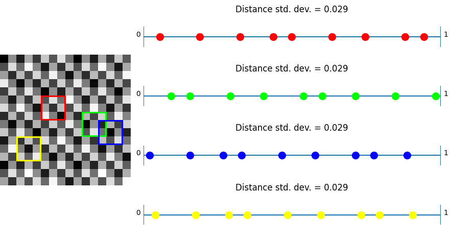
IGN is low discrepancy in a different sort of way. If you look at any 3×3 block of pixels, even overlapping ones, you will find that the 9 values roughly match all values 0/9, 1/9, 2/9, … , 8/9, but that they are a bit randomized from the actual values. Every 3×3 block of pixels makes a low discrepancy set on the 1D number line.
Let’s pick a couple blocks of pixels and look at the distance between values in those pixels. First is IGN, which has a very low, and constant, standard deviation. The values are well spaced.
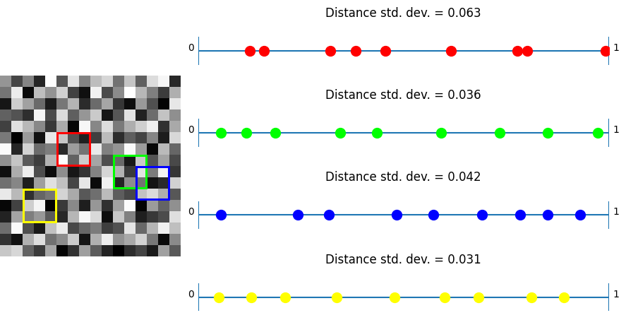
Here is white noise which has clumps and voids so has very high variance in distance between values:
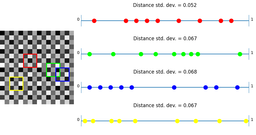
Here is blue noise which does a lot better than white noise, but isn’t as good as IGN.
Lastly here is Bayer which is better than white noise, but is still pretty clumpy.
How Does IGN Make TAA Work Better?
TAA, or temporal anti aliasing, tries to make better renders for cheaper by amortizing rendering costs across multiple frames. Why take 10 samples in 1 frame, when you can take 1 sample for 10 frames and combine them?
The challenge in TAA is that objects are often moving, and so is the camera. You can use the current frame’s camera matrix, the previous frame’s camera matrix, and motion vectors to try and map pixels between frames (called temporal reprojection) but there are times when objects become occluded, or similar events that cause the found history to actually be invalid. If you don’t handle these cases and throw out the invalid history, you get ghosting where pixels use invalid history.
A common way to handle the problem of ghosting is to make a minimum and maximum RGB color cube of the 3×3 neighboring pixel colors for the current frame of a pixel, and clamp the previous frame’s pixel color to be inside of that box. The clamping makes any history which is too different be much closer to what is expected. The previous frame’s clamped pixel color is then linearly interpolated towards the current frame’s pixel color by a value such as 0.1. That leaky integration is called “Exponential Moving Average” which allows a running average that forgets old samples over time, without having to store the previous samples.
When TAA samples the 3×3 neighborhood, the intent is to get an idea of what possible colors the pixel should be able to take, based on the other other pixels in the local area. The more this neighborhood accurately represents the possible values of pixels in this local area, the more accurate the color clipping history rejection will be. IGN makes the local area more accurately represent the full set of possibilities in small neighborhoods of pixels.
For instance, let’s say you had a bright magenta object in front of a dark green forest background, and you were using stochastic alpha to make the magenta object be semi transparent. That is, the bright magenta object may have an opacity of 0.1111… (1/9) so using a random number per pixel in this object, you’d let 1/9th of the pixels be written to the screen, while 8/9ths of them would be discarded.
Ideally, you’d want every 3×3 block of pixels in this magenta object to have a single magenta pixel surviving the stochastic alpha test so that the neighborhood sampling would see that magenta was a possibility, and to keep the previous pixel’s history instead of rejecting it, allowing the pixel to converge to 1/9th transparency better.
With white noise random numbers, you would end up with clumps of magenta pixels and voids where they should be but aren’t. This makes TAA reject history more often than it should, making for a worse, less converged result.
With IGN, every 3×3 block of pixels (even overlapping blocks) has a low discrepancy set of scalar values, so you can expect that out of every 3×3 block of 9 pixels, that 1 pixel will survive the stochastic alpha test. This is how IGN improves rendering under TAA.
Blue noise sort of has this property, but not as much as IGN does. Bayer looks like it has this property but the regular grid of the result isn’t good for diagonal distances, while also looking more artificial.
Stochastic transparency using various per pixel noise types. The object has 1/9th transparency. Friends don’t let friends use white noise!
In other situations where you need a per pixel random number, results like the above will normally hold as well (small regions of pixels will more accurately represent all the possibilities), this isn’t limited to stochastic alpha.
Derivation Of IGN And Extensions
If you were to sit down to make IGN you might define your constraints as: “Every 3×3 block of pixels in an infinite texture should have the values 1 through 9”. At this point, you’ve basically described sudoku. If you then go on to add “Also, this should include OVERLAPPING blocks”, you’ve made a generalized sudoku. It turns out this is too many conflicting constraint and is not solvable. A way to get around this problem would be to put a little bit of drift in the numbers over space so that it was mostly solved and the error of the imperfect solution was distributed over space. At this point, you have reached how IGN works.
I asked Jorge how he made IGN and it turned out to involve spending a full 8 hour day (or was it longer? I forget!) sitting at a computer tweaking constants by hand until they had the properties he was looking for. That is some serious dedication!
float IGN(int pixelX, int pixelY, int frame)
{
    frame = frame % 64; // need to periodically reset frame to avoid numerical issues
    float x = float(pixelX) + 5.588238f * float(frame);
    float y = float(pixelY) + 5.588238f * float(frame);
    return std::fmodf(52.9829189f * std::fmodf(0.06711056f*float(x) + 0.00583715f*float(y), 1.0f), 1.0f);
}
If you are wondering how you might be able to make vector valued IGN, we did that in our spatiotemporal blue noise work by putting the scalar IGN values through a Hilbert curve. The scalar value was multiplied (and rounded) to make an integer index, and that was put into the Hilbert curve to make a vector out. When we used those vectors for rendering, the resulting noise in the render was very close to scalar IGN. There are probably other methods, but this ought to be a good starting point.
Proposed Terminology: Low Discrepancy Grids
Low discrepancy sequences are ordered sequences of scalar or vector values. They are a function that looks like the below, with index being an integer, and value being a vector or a scalar:
IGN works differently though. You plug in an integer x and y pixel coordinate and it gives you a floating point scalar value.
Or in C++:
float IGN(int pixelX, int pixelY);
Low discrepancy sequences are in contrast to Low discrepancy sets. Sequences have an order, and taking any number of the values starting at index 0 will also be low discrepancy. Low discrepancy sets don’t have an order, and should only be expected to be low discrepancy if all the values in the set are considered together.
Other terminology calls low discrepancy sequences “progressive” and low discrepancy sets “non progressive”.
So what should we call IGN or similar noise functions that take in a multi dimensional integer index and spit out a scalar value? There is definitely an ordering, so it isn’t a set, but the ordering is 2 dimensional and there really isn’t a starting location, since negative numbers work just as well as positive numbers in the formula.
I propose we should refer to them as low discrepancy grids. That would cover the various types of grids: regular, irregular, skewed, curvilinear, and beyond, and these in any dimension. IGN itself more specifically would be a low discrepancy regular grid, or a low discrepancy cartesian grid.
Interleaved Gradient Noise is a very interesting noise pattern for use with per pixel random numbers, optimized towards neighborhood sampling rejection based TAA.
Even though it isn’t as widely known or understood as it should be, a secondary value to this work is showing that per pixel random numbers / sampling patterns can be generated for specific needs with great success.
This concept, along with the importance sampled vector valued spatiotemporal blue noise work recently put out are just two instances of this more general concept, and I believe they are just the beginning of other things yet to be created.