An irrational number is a number that can’t be represented as a fraction using integers for the numerator and denominator.

I’m a big fan of irrational numbers, and one of the biggest reasons for that is that they are great at making low discrepancy sequences, which give amazing results when used in stochastic (randomized) algorithms, compared to regular random numbers. Low discrepancy sequences are cousins to blue noise because they both aim to keep samples well spread out, but the usage case is different, so it’s situational whether to use blue noise or an LDS. That means that luckily there is room enough in the world for both LDS and blue noise.

This post is a random grab bag of things relating to irrational numbers.

Pythagorian cultists supposedly murdered someone to keep irrational numbers a secret, so this is technically forbidden knowledge, I guess.

Making Continued Fractions – Pi and Milü

Continued fractions are a way of writing numbers that can be useful for helping analyze irrational numbers, and rational approximations to specific numbers – whether they are rational or irrational.

If a continued fraction is infinitely long, that means it represents an irrational number, and all irrational numbers have continued fractions that are infinitely long. If a continued fraction is not infinitely long, that means it’s a rational number.

Here is the beginning of the continued fraction for pi.

Another way of writing continued fractions is to get rid of all the redundant “1 divided by…” and just write the integers you see on the left. The continued fraction for pi above would look like this, which is a lot more compact:

[3;7,15,1,292,1,1,1,2,1,3,1]

Let’s talk about how you make a continued fraction by walking through how to make it for pi, or at least 3.14159265359 anyways, since pi goes forever.

First up you take the integer part and use that as the first digit. Subtracting that integer part out leaves you with a remainder:

[3]
remainder: 0.14159265359

We take 1/remainder to get 7.06251330592. The integer part of this number is going to be our next number. Subtracting the integer part out gives us our next remainder:

[3;7]
remainder: 0.06251330592

1/remainder is 15.9965944095, which makes our next integer and remainder into:

[3;7,15]
remainder: 0.9965944095

1/remainder is 1.00341722818, so now we are at…

[3;7,15,1]
remainder: 0.00341722818

1/remainder is 292.63483365 so now we are at:

[3;7,15,1,292]
remainder: 0.63483365

1/remainder is 1.57521580653 and we’ll stop at the next step:

[3;7,15,1,292, 1]
remainder: 0.57521580653

Wherever you have a large number in the continued fraction, it’s because you just did one divided by a small number. The larger the integer means the smaller the remainder there was to make that integer.

The smaller a remainder is, the better approximated the number is at that step of the continued fraction.

This means that when you see a large number in a continued fraction, that if you truncated the continued fraction right before that large number, you’d have a pretty good approximation of the actual number that the continued fraction represents.

The larger the number, the better the approximation.

Because of this, looking at the continued fraction for pi, below, you can see that it has a pretty large number (292) pretty early in the sequence.

[3;7,15,1,292,1,1,1,2,1,3,1]

This means that the following continued fraction approximates pi “pretty well”.

[3;7,15,1]

We’ll cover how to figure this out further down in the post, but that fraction is actually 355/113 and has a special name “Milü”, found by Chinese mathematician and astronomer, Zǔ Chōngzhī, born 429 AD. It is within 0.000009% of the value of pi.

More info from wikipedia: https://en.wikipedia.org/wiki/Mil%C3%BC

So, while pi is probably the most famous irrational number, it certain isn’t the most irrational number that there is, as it is so easily approximated by smallish integers in a division.

Quick note if you write a program to convert a floating point number to a continued fraction: If you try to make a continued fraction for a number that a floating point can’t represent exactly – such as 4.1 – you will get a very tiny remainder which then makes a very large integer when you flip it over. In my case, when using doubles, it made such a large number that converting it to an integer overflowed the integer. One way to address this is to just consider any remainder smaller than some threshold as zero. Like maybe any remainder less than 0.00001 can be considered zero.

The Continued Fraction of Phi aka The Golden Ratio

So even though pi is not the most irrational number, phi is (pronounced “fee”, and is aka the golden ratio). Yes, it is the most irrational number!

We’ll use the value 1.61803398875 and make a continued fraction.

[1]
remainder: 0.61803398875
1/remainder: 1.61803398875

[1;1]
remainder: 0.61803398875
1/remainder: 1.61803398875

[1;1,1]
remainder: 0.61803398875
1/remainder: 1.61803398875

Wait a second… do you see a pattern? the remainder is always the same value, and then when we do 1/remainder we always get the golden ratio again. That means this continued fraction is 1’s all the way into infinity.

In the last section we saw how having a large number in the continued fraction meant that a number was well approximated at that point in the continued fraction.

The golden ratio has a 1 for every number in the continued fraction, which is the smallest value you can have. That means it’s as least well approximated as you can be, at every stage in the continued fraction.

This is what is meant by the golden ratio being the most irrational number. It’s the least well approximated by rational numbers (dividing one integer by another).

When I said I liked irrational numbers I was mainly talking about the golden ratio, but other highly irrational numbers, like the square root of 2, are also nice. Highly irrational numbers have the properties that I like – the properties that make them useful to use as low discrepancy sequences.

An interesting thing you may have noticed above is that when you divide 1 by the golden ratio, you get the golden ratio minus 1. That is:

1 / 1.61803398875 = 0.61803398875

If you replace the golden ratio with “x” you get this equation:

1/x = x-1

If you solve that equation, you will get the golden ratio out. It is the only number that has this property! Well actually, -0.61803398875 does too, and relates to the fact that there is a + and – root solution to that quadratic equation, but maybe that’s not that surprising. 1/-0.61803398875 is -1.61803398875. The behavior is the same, it’s just happening on the other side of zero.

Something else interesting about the golden ratio is that if you square it, it’s the same as adding 1.

1.61803398875*1.61803398875=2.61803398875

That gives you a formula:

x*x = x+1

If you solve that, you get the golden ratio again as the only solution (well, and the negative golden ratio minus 1 just like before). Probably not too surprising if you look at the formulas though, as you can use simple algebra to change one formula into the other.

From Continued Fractions To Regular Fractions

If you had a continued fraction and wanted to turn it into a regular fraction (or real number), you could run the process in reverse.

However, doing that means you start at the right most digit of the continued fraction and work left til you get to the beginning. How do you do this with an infinitely long continued fraction, like an irrational number would have?

Luckily there is a way to start at the left and work right, so that you can get approximations to infinitely long continued fractions (irrational numbers).

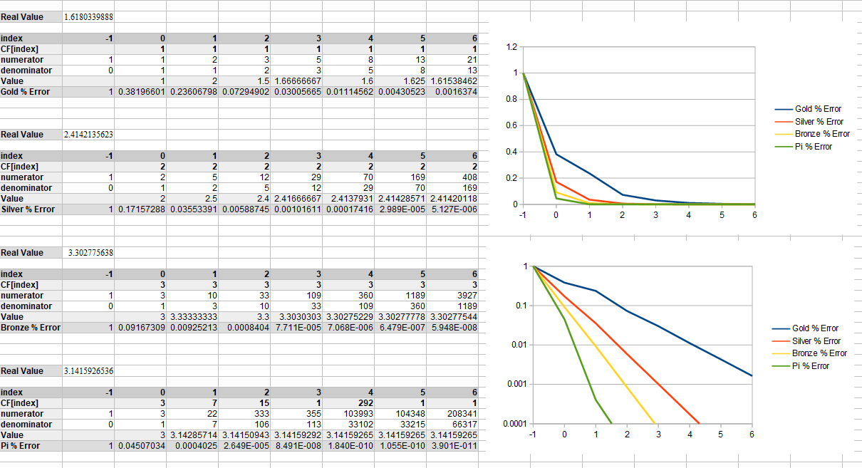
Let’s do this with pi, with this much of the continued fraction:

[3;7,15,1,292,1,1]

What you do is make a table which has a row for the numerator and denominator. The first numerator is 1, and the first denominator is 0. The second numerator is the first number in the continued fraction sequence, and the second denominator is 1.

The formula for the rest of the numerators and denominators is…

• numerator[index] = CF[index] * numerator[index-1] + numerator[index-2]
• denominator[index] = CF[index] * denominator[index-1] + denominator[index-2]

Doing that from left to right, you get this:

Below we do that with pi, golden ratio, sqrt(2) and an irrational number i came up with that is not very irrational, and is well approximated by 1.01.

A quick fun tangent is that you might notice that for golden ratio, both the numerators and denominators are the Fibonacci numbers. This is the link between the golden ratio and Fibonacci numbers.

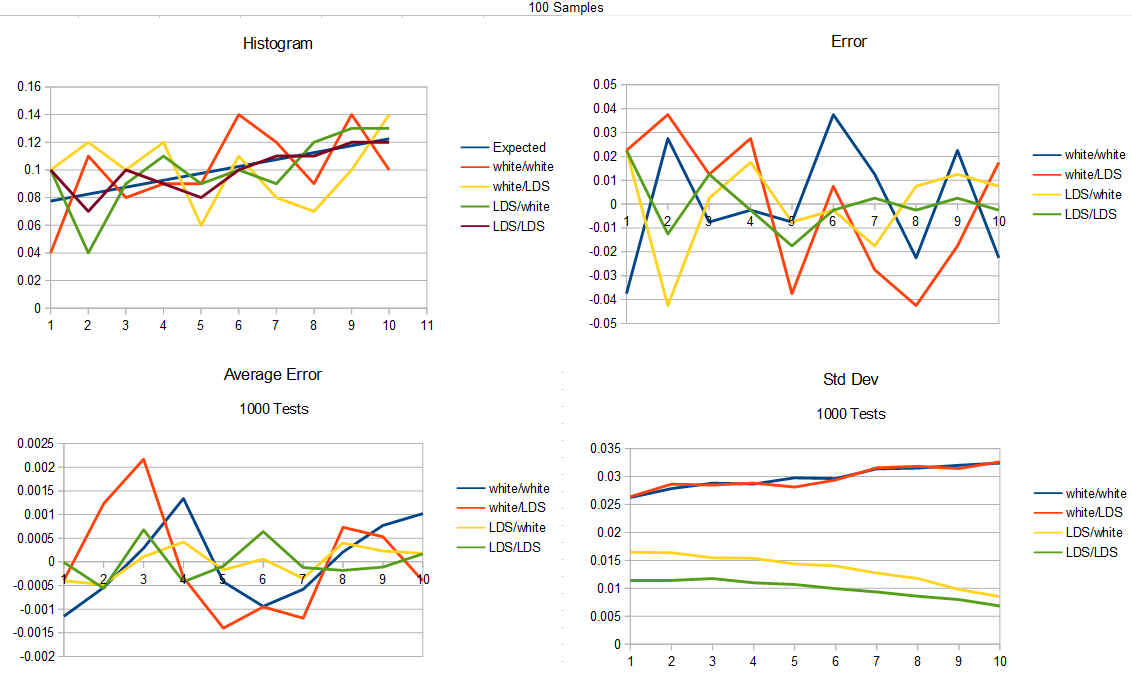
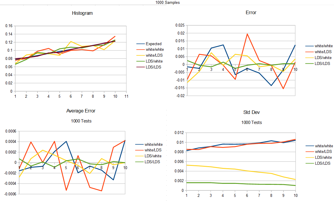
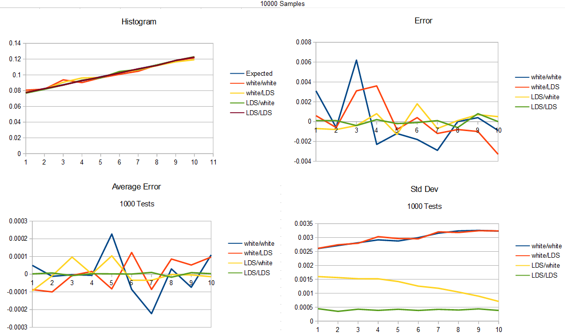
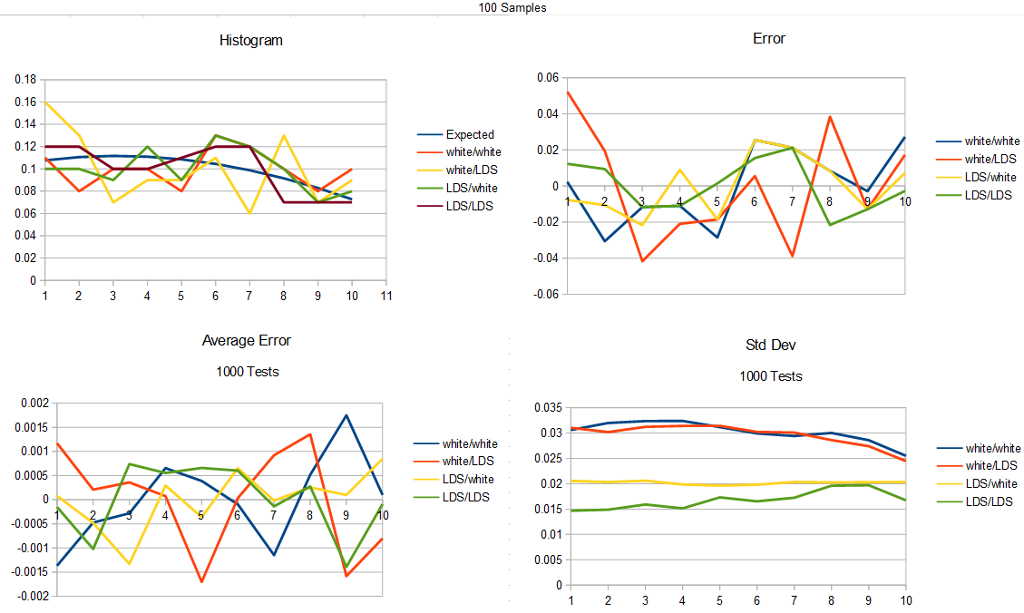
Below shows the percentage error of each number, as more terms in the continued fraction are added.

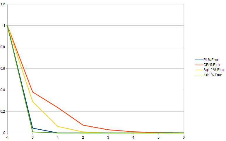
Golden ratio error decreases the slowest which shows that the golden ratio is least well approximated by fractions. The made up irrational number that is approximately 1.01 has error decreasing the fastest because it is the least irrational of these numbers. Pi shows itself as having fairly low irrationality, and the square root of 2 is fairly irrational.

Here is the error on a log y axis to better show the difference in error.

It’s worth noting that 1/goldenRatio aka 0.61803398875 is every bit as irrational as the golden ratio itself is. The reason for this is that we are flipping the numerator and denominator over for this fraction that doesn’t exist. Flipping it over doesn’t make it more representable as a fraction.

When I’m using the golden ratio for low discrepancy sequences, i usually use that 1/goldenRatio value, also known as “the golden ratio conjugate” because the smaller value means it’s going to have fewer numerical issues and more precision, when working with small values (like between 0 and 1).

Also, there are an infinite amount of numbers just as irrational as the golden ratio. You can calculate them by calculating:

where p,q,r,s are integers and the absolute value of p*s-q*r is 1.

That is the Moebius transform.

If you are wondering what the least irrational number is, it looks like there are multiple (infinite) and they are just numbers that are very, very, very well approximated by rationals. They are called Liouville numbers and are transcendental, meaning they can’t be calculated with polynomials basically. Proving the existence of these numbers also probed the existence of transcendental numbers themselves. (https://en.wikipedia.org/wiki/Liouville_number)

There is also something called an irrationality measurement, but I haven’t found it that useful. It doesn’t seem to be something you can calculate with a program and compare two numbers to see which is more irrational. https://mathworld.wolfram.com/IrrationalityMeasure.html

Metallic Means

If all 1’s in a continued fraction make the golden ratio, what would all 2s or all 3s make? That makes the silver and bronze ratio respectively and all three of these are the first three of the “Metallic Means”. You can see the details of them below, along with pi. Wikipedia talks more about them too at https://en.wikipedia.org/wiki/Metallic_mean

You might also be interested in reading about the “Plastic Number” which is a different way of trying to approach the goodness of the golden ratio to get another decently irrational number. https://en.wikipedia.org/wiki/Plastic_number

Where the golden ratio has a formula x^2 = x+1, the plastic number has a formula x^3 = x+1.

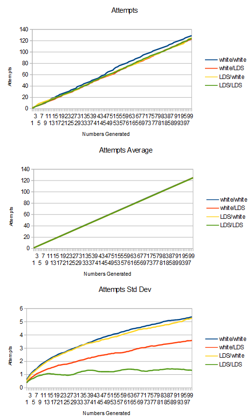
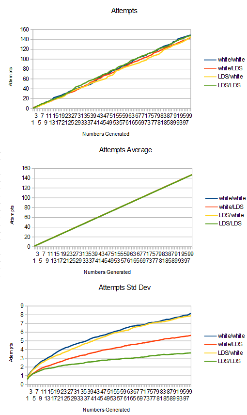
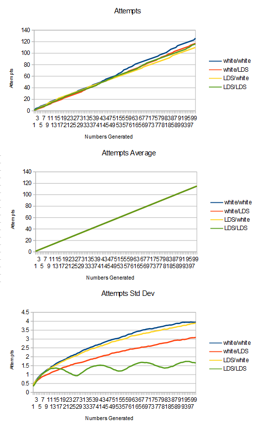
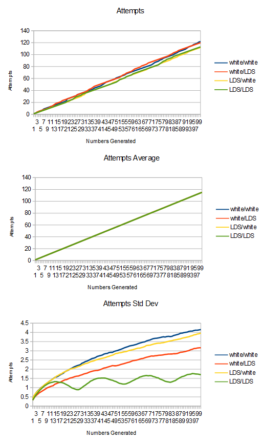
Coprime Numbers (Setup For Irrational LDS)

Coprime numbers are 2 or more integers that share only 1 as a factor.

For instance, 7 and 11 are coprime numbers. They also happen to be prime numbers, but coprime numbers don’t have to be prime. 8 and 15 are also coprime numbers although neither number is prime. You can even lump all four together and say that 7, 8, 11, 15 are coprime numbers. Combining lists of coprime numbers doesn’t usually result in a list of numbers that are still coprime. This just worked out because we added only prime numbers to the other list of coprimes, and adding primes will always keep the list of numbers coprime.

You might wonder why you should care about coprimes.

My favorite use of coprimes is when i need cheap shuffles of numbers.

For instance, let’s say you had 8 numbers and you wanted them to be shuffled into a somewhat randomized order, but it didn’t need to be a very high quality shuffle.

What you do is first pick any number that is coprime to 8… we’ll say 5. You then count an index from 1 to 8 and do this…

Out = (index * 5) % 8

Taking index from 1 to 8 gives you the following output:

5, 2, 7, 4, 1, 6, 3, 0

If you look at it a bit, you can probably find some patterns, but all the numbers are there and it is fairly mixed up wouldn’t you say? A casual observer probably isn’t going to notice any patterns if you used this in a game setting for dropping treasure or something.

Not all coprime choices give the same quality results though. Here is what happens if we use 7 as the coprime number instead of 5:

Out = (index * 7) % 8

7, 6, 5, 4, 3, 2, 1, 0

It just reversed the list! That isn’t very mixed up.

Also, let’s look at what happens if you don’t use coprimes. We’ll use 2 instead of 7.

Out = (index * 2) % 8

2, 4, 6, 0, 2, 4, 6, 0

If the numbers aren’t coprime, it won’t generate all the numbers in the list. Another way of looking at this is that the cycle length of the number sequence is maximally long when the numbers are coprime, but are not going to be as long (and will repeat) if the numbers are not coprime.

Note that you don’t have to use index values 1 through 8. You could use 0 through 7 instead or any other contiguous 8 values – like 127 through 134. The numbers in this case are all mod 8, so 127 through 134 is equivalent to 7 through 14.

Irrational LDS

An additive recurrence sequence is basically the same concept as the last section, but taken to the continuous world instead of sticking to discrete integers. You use the formula below, where A is any real number:

Out = (index * A) % 1

Just like before with coprime numbers, the value you multiply index by can make you have better or worse results.

If you pick 1/2 (0.5) for A, the sequence you’ll get out is this:
0.5, 0.0, 0.5, 0.0, 0.5, …

If you pick 1/4 (0.25) for A, you’ll get this:
0.25, 0.5, 0.75, 0.0, 0.25, 0.5, 0.75, 0.0, …

1/3 will get you this:
0.333, 0.666, 0.0, 0.333, 0.666, 0.0, …

2/3 will get you this:
0.666, 0.333, 0.0, 0.666, 0.333, 0.0, …

You can also do something more complex, like 5/8:
0.625, 0.25, 0.875, 0.5, 0.125, 0.75, 0.375, 0.0, …
(it then repeats)

If we picked 2/4, we’d end up with 0.5, just like we did when we used 1/2. When thinking about fractions to use in this setup, you should reduce the fraction, because unreduced fractions give the same value as reduced fractions. Ready for the kicker? The numerator and denominator in a reduced fraction will always be coprime integers – by definition of being a reduced fraction! Also, the denominator of the reduced fraction will tell you the length of the sequence it generates.

I snuck a little trick in the examples, did you catch it?

Let’s look at that sequence using 5/8 again, but let’s write the results as fractions.

5/8, 2/8, 7/8, 4/8, 1/8, 6/8, 3/8, 0/8, …

Now let’s look back at the sequence we made last section where we did (index*5)%8

5, 2, 7, 4, 1, 6, 3, 0

The numerator in the fraction results is the same as the integer one using coprimes. You could multiply the fractional results by 8 and get the exact same numbers. In fact take the formula we are using in this section:

Out = (index * 5/8) % 1

And multiply it by 8 to get the formula used in the last section!

Out = (index * 5) % 8

So, while we seemed to have moved away from integers into a continuous domain, we haven’t really… we are still in the land of coprime number sequences. We will always be in the land of coprime number sequences as long as we are using rational numbers, because there will always be a coprime numerator and denominator pair in the simplified fraction that defines the length of the sequence that comes out when we feed index numbers in.

So what if we ditch rational numbers and go with an irrational number? Well, using an irrational number means that the sequence will never repeat. While that in itself sounds awesome, let’s imagine we are using an irrational number that is well approximated by 1/4. That means that the sequence would never repeat, but it would NEARLY repeat every 4 values.

Let’s show the sequence using the golden ratio, where index goes from 1 to 8.
0.618034, 0.236068, 0.854102, 0.472136, 0.090170, 0.708204, 0.326238, 0.944272

Here is the same for a not very irrational number that we are going to approximate with 0.2490001.
0.249000, 0.498000, 0.747000, 0.996000, 0.245000, 0.494001, 0.743001, 0.992001

You can see that the sequence with the ~0.25 irrational isn’t EXACTLY repeating, but it sure is close to repeating. The golden ratio is making very unique numbers in comparison

So basically, if you use an irrational number that can be closely approximated by a rational number, it’ll behave a lot like that rational number and not be real great.

This is what is great about the golden ratio and other highly irrational numbers. There is no rational number that well approximates them, so not only do they not have any actual repeats, they also don’t have any NEAR repeats.

Using highly irrational numbers in this additive recurrence formula, you get a low discrepancy sequence.

Irrational LDS Offset

Every time you use an irrational LDS, you are going to get the same sequence, which can sometimes be a problem.

You can get around this by starting at a different index every time, or by adding a different starting value to the sequence.

Option #1: Randomized Start Index:

Out = ((index+StartIndex) * Irrational) % 1

Option #2: Randomized Starting Value:

Out = (Index * Irrational + StartValue) % 1

How you get this starting index or starting value is up to you. Honestly, I use white noise random numbers and it works fine, so I’ll keep doing that until I analyze it and find out how much better using an LDS is.

Anyways, if you recall from earlier in the post, this LDS won’t repeat so long as you use an irrational number. That means that the infinite number of integer index values going in means you get an infinite number of unique real numbers coming out. That means that the LDS can output any number possible just by changing the index you are at. So, offsetting by index is equivalent to offsetting by a start value, since there is some index that should give the same output as any specific starting value.

I thought that was true, but it turns out it isn’t, because integers are countably infinite while irrational numbers are a larger infinity.

It turns out that this is nearly true though, and that there always exists an index that will give you a value arbitrarily close to any specific starting value.

Although, this is only mathematically true. Computers have finite storage for integers and floats.

Anyways, it’s complicated, but either offsetting index or starting value should work just fine for getting a different sequence. I go the starting value way myself.

More info here regarding that mathematical topic: https://twitter.com/Atrix256/status/1285646721561899010?s=20

BTW even though i show the formula for irrational LDS as index multiplying by the irrational number, that will have numerical precision problems as the index gets larger. You are way better off just adding the irrational and doing modulus when you want the value for the next index. The difference is huge, surprisingly!

Irrational LDS & Arbitrary Start Progressive Sequences

There is the concept of a progressive low discrepancy sequence, which means that any subset of the sequence, starting at index 0, will have the same properties as the entire sequence.

For instance, if you had a progressive blue noise sequence with 100 samples in it, using only the first 10 samples would be blue noise, or using the first 47 samples, or the first 73, or all 100.

If you had a non progressive blue noise sequence, the sample sequence wouldn’t be blue noise until all 100 samples have been used (or as you got close to that number).

Irrational low discrepancy sequences have a nice property that they are progressive, and they are progressive starting at ANY index, not just from index 0. This is because offsets in index are roughly equivalent to offsets in starting value, so starting in the middle of the sequence is the same as if you just started with that sample’s value as the starting value.

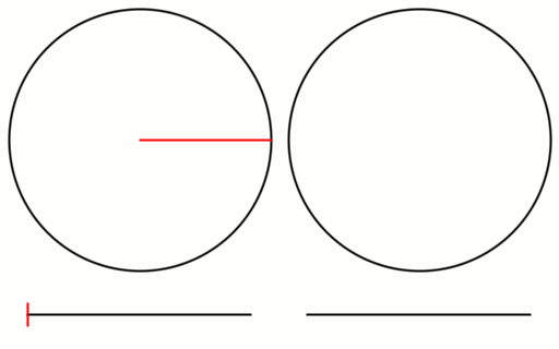
The golden ratio in particular is great for this. Each new sample from the golden ratio LDS falls in the biggest hole left by samples so far, which is why it’s so great for numerical integration (and similar). It has great coverage over the sampling domain. The crazy thing though, is that you can start at any index in the LDS and this is still true from that starting index, while it’s still also true if starting from index 0.

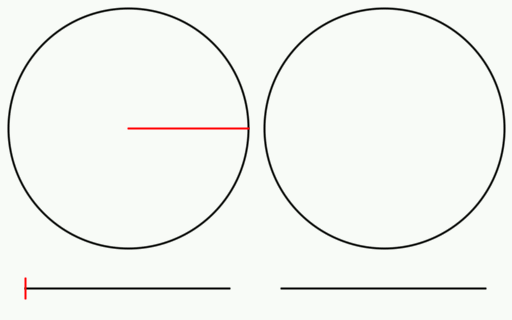
Check out the gif below to see what i’m talking about. There are 16 samples total. All 16 are shown on the left, but only the last 8 are shown on the right. I show the samples on a numberline since they are scalar values between 0 and 1, but I also show them on a circle to see that what i said about falling in the largest gap is true even with wrap around.

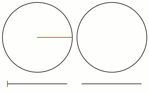
Here is the same setup for an animation using the square root of 2 instead.

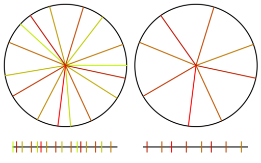
Lastly, here is the same with pi. Pi is well approximated by 22/7 and since we are walking around a circle, the integer parts are irrelevant. Since 22/7 is 3 1/7, that makes pi act nearly like 1/7 and you can verify that it is indeed nearly repeating every 7 samples, and acting very much like 1/7. You can see how pi has samples that clump and it doesn’t give very good coverage over the sample domain for the number of samples it uses (compare the coverage to golden ratio!). This shows how a less irrational number isn’t as good at being a low discrepancy sequence.

If you have heard that plants grow leaves in a golden ratio pattern, now is probably a good time to explain why. Here is the last frame of the golden ratio gif, when there are 16 samples.

One of a plant’s goals in life is to get as much sun as it possibly can. Imagine that the sun is directly overhead and you are looking down at the plant from above. Toward this goal of maximizing sunlight, whenever light is allowed to hit the ground in the radius of the circle of the plant’s shadow, that is a lost opportunity. Sunlight is being wasted by hitting the dirt.

There may also be temporary or semi-permanent shadows that exist or come into existence at any point in the plants life, and if it put all it’s leaves such that they clump in one direction, all those leaves may become in shadow and the plant could go hungry.

A solution to these problems is to grow leaves equally distributed around the plant. This way there are no overlaps when viewing from above, and the risk of shadowing is minimized by being well spread out over all directions.

This would be the end of it if a plant was born with all of it’s leaves and it knew how many leaves it was going to need to grow – and that no leaves were going to get eaten.

Plants are dynamic life forms though, in a dynamic environment, so the leaves need to be as evenly spaced radially as possible when it’s a seedling with just a couple leaves, but also when it is much older with many leaves, possibly with some of them eaten by animals, and all that jazz.

A good way to do this would be to use the golden ratio to figure out where the grow the next leaf.

Doing this, it will have good coverage over the entire circle of possible growth, it’s ok if old leaves die off and go away since it will still be well distributed, leaves can grow larger because overlap will be minimized.

Check out the gif again and think of each line as a leaf growing around a central stem, as the plant gets taller. The circle on the right shows what happens as the first 8 leaves get old, die and fall off, being replaced by 8 new leaves.

If this talk about plants was interesting, give a read here about “Phyllotaxis”
https://en.wikipedia.org/wiki/Phyllotaxis

A Connection Between Primes and Irrationals

So when we have this function where Out, A, B and index are integers:

Out = (index * A) % B

We will get a non repeating sequence of numbers B long from 0 to B-1, if A and B are coprime. Since prime numbers are coprime with all other numbers, we could also say that if A is prime, the sequence will have those properties. It isn’t required to be prime (just coprime) but let’s make the statement for primes right now.

If we move that to the real number world, where index is an integer, but A and out are real numbers:

Out = (index * A) % 1

If A is irrational, we will get a non repeating sequence of numbers infinitely long. In that way, irrational numbers are like primes in that when used, they make a non repeating sequence that is as long as possible.

More so, as A is more highly irrational, you get fewer “near repeats” as well, until getting to the golden ratio where you get a provably minimum amount of near repeats.

So, primes and irrationals (especially the golden ratio), are linked in that they make maximal length non repeating sequences when used over a field.

Co-Irrational Numbers

We talked about coprime numbers and how they would make a sequence that “went the full length”, that is, they made a sequence that didn’t repeat over the whole sequence. If you multiplied index by 5 and did a modulus by 8, you would get a sequence that was 8 items long and then would repeat.

We also talked about irrational numbers and how they would make sequences that NEVER repeated, and talked about how highly irrational numbers could make sequences that also didn’t have NEAR repeats.

This is great if you want one dimensional sequences, but what if you want two dimensional sequences or higher?

One way to do higher dimensional low discrepancy sequences is to just use a different irrational number per axis.

That is great but now you find yourself having to come up with a bunch of high quality irrational numbers since you need one for each axis. Sadly, there is only a single “golden ratio” really (Moebius transform and conjugate don’t give different behavior). If you used the golden ratio on each axis, you’d have correlation between the axes and it wouldn’t be great. Basically, each axis would have the same pattern, even if you start at a different index, or starting value.

There’s a concept I’m sure someone has thought of before, maybe going by a different name, that I call “co-irrationality”.

Coprime numbers have no shared factors other than 1, and thus “no shared cycle lengths” which make their output sequences be maximal lengths.

Similarly, co-irrational numbers should minimize how close they get to each other with their rational approximations. Where non coprime numbers used to make a sequence will repeat, two numbers that aren’t very co-irrational will make a sequence that will nearly repeat, which is nearly just as bad.

Just like how a coprime number doesn’t have to be prime, a co-irrational number doesn’t have to be very good as an irrational number in itself, and in fact, a rational number and irrational number could together be “co-irrational” to each other (like the golden ratio and 2). Also, you could have more than 2 numbers in a set that are co-irrational to each other.

The question of whether two or more numbers are coprime results in a black and white answer: a yes or a no.

The question of whether two or more numbers are co-irrational results in a grey answer. Numbers can range from not being co-irrational at all (if one is a multiple of the other), to being various levels of co-irrational, up to maximally co-irrational (again, the example of the golden ratio and 2).

So how can you tell if two numbers are co-irrational, or rather, how co-irrational they are?

Basically, divide one number by the other (doesn’t matter which is the numerator and which is the denominator) and then look at the irrationality of the resulting number. If the result is a rational number, the numbers are not co-irrational. If the result is an irrational number that is well approximated by dividing relatively small integers, the numbers are not very irrational. If the result is the golden ratio, the numbers are maximally irrational.

If you wanted to see how co-irrational 3 or more numbers were, one way could be to look at them pair-wise. You’d have to figure out how to combine the results of the multiple tests since you are testing each possible pair, but it should give you an idea of how co-irrational they were.

This might also give some thoughts on how you could come up with a set of N co-irrational numbers. Maybe gradient descent could be used to find N numbers that when looked at pairwise, gave the results closest to the golden ratio, and made the error be evenly split up between the pairs.

This section is light on evidence / experimentation / etc, but the post is already getting pretty long. It could be fun to look more deeply at co-irrationals in a separate post.

Super Golden Ratio

Apparently there is a super golden ratio. Image below taken from this video: https://www.youtube.com/watch?v=X9DpdomPRvg
There is a short video here talking about some of it’s properties: https://www.youtube.com/watch?v=A4cN_44VOfQ

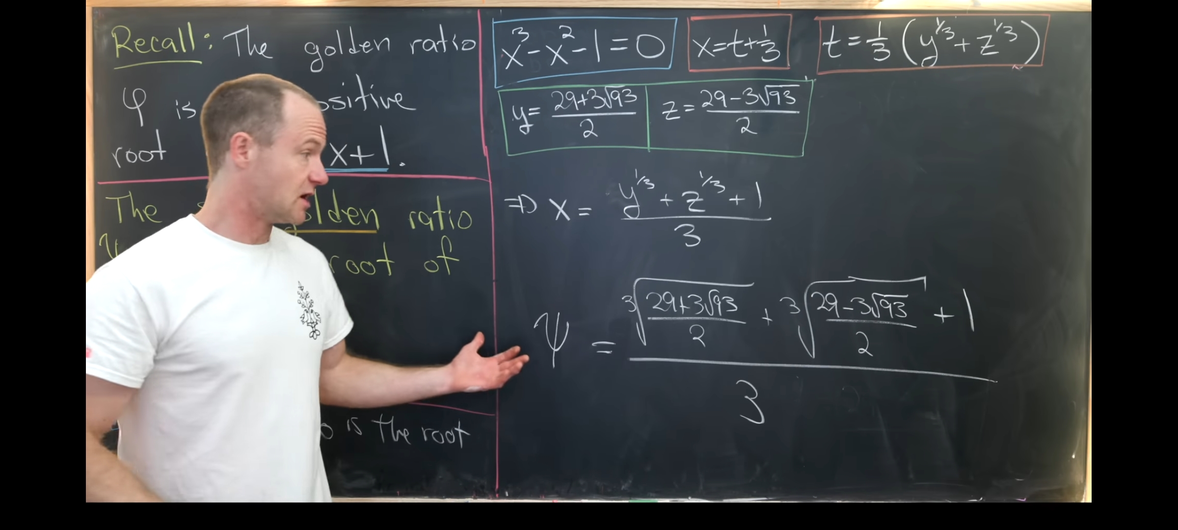
Analyzing the super golden ratio, it isn’t as irrational as the golden ratio, but it makes me curious what it might be useful for.  If you find or can think of anything, I’d love to hear about it!

Here is the C++ code to calculate it that you can copy & paste

static const double c_superGoldenRatio =
(
std::pow((29.0 + 3.0 * std::sqrt(93.0)) / 2.0, 1.0 / 3.0) +
std::pow((29.0 - 3.0 * std::sqrt(93.0)) / 2.0, 1.0 / 3.0)
+ 1.0
)
/ 3.0;

Here is the continued fraction:

1.465571 = [1, 2, 6, 1, 3, 5, 4, 22, 1, 1, 4, 1, 2, 83, 1, 1, 1, 25, 11, 1]

Here is the same test done as before on the circle and number line.

Links

This is a really great read by Martin Roberts (https://twitter.com/TechSparx) talking about generalizing the golden ratio and using that generalization for multi dimensional low discrepancy sequences, that is competitive with Sobol.
http://extremelearning.com.au/unreasonable-effectiveness-of-quasirandom-sequences/

This talks about whether adding irrational numbers together or multiplying them together results in an irrational number:
https://mathbitsnotebook.com/Algebra1/RatIrratNumbers/RNRationalSumProduct.html?s=09

This talks about how we know that e+pi is irrational or e*pi is irrational, or both, but that’s all we can say about it:
http://mathforum.org/library/drmath/view/51617.html

This shows a link between primes, Pascal’s triangle, and constructable polygons:
https://en.wikipedia.org/wiki/Constructible_polygon

Here is an alternate take on how to measure co-irrationality:
https://twitter.com/R4_Unit/status/1284588140473155585?s=20

Legend has it that a man named Hippasus was killed by Pythagorean cultists for proving the existence of irrational numbers, which destroyed their world view that all numbers were rational.

Here’s a video about that:
https://www.youtube.com/watch?v=sbGjr_awePE

Here’s an article:
https://nrich.maths.org/2671

Here’s another article:
http://kiwihellenist.blogspot.com/2015/11/were-greeks-scared-of-irrational-numbers.html

And another:
https://io9.gizmodo.com/did-pythagoras-really-murder-a-guy-1460668208

Numberphile has a nice video on the irrationality of phi too: https://www.youtube.com/watch?v=sj8Sg8qnjOg

The code that generated the data for this post & implements the things talked about can be found at: https://github.com/Atrix256/LDSRejectionSampling

Rejection sampling lets you convert numbers from one probability distribution into numbers from a different probability distribution. It does that by throwing numbers away.

Imagine I gave you one hundred binary digits where 50% were zeros and 50% were ones. If you wanted them to be 75% zeros and 25% ones you could throw away 33 of the ones. That would leave you with 67 numbers where 50 were zeros and 17 were ones. Now, 74.6% of the numbers are zeros, and 25.4% of the numbers are ones. The transformation worked.

That change in distribution came at a cost though, the sequence got smaller.

I previously wrote up a post about rejection sampling here:
Generating Random Numbers From a Specific Distribution With Rejection Sampling

I also wrote about inverting a CDF here, which is a more complex method where you don’t throw numbers away.
Generating Random Numbers From a Specific Distribution By Inverting the CDF

When doing rejection sampling, a random number is compared against the probability for a number to survive, and the number is thrown away if it fails that test.

This post is going to look at what happens if we use low discrepancy sequences instead of random numbers (white noise) when working with rejection sampling. We are going to try substituting LDS for the random number generation to see if we should throw away a sample, and also we are going to use an LDS to generate the sequence we use as the source of rejection sampling.

Why LDS Here?

You might be asking what the motivation is for trying low discrepancy sequences here.

As a general rule, whenever I see white noise (regular random numbers) being used, it’s usually an indication that money is being left on the table and that the situation could be improved by using something else.

My heuristic there is roughly that if it’s for graphics, with sample counts that aren’t going to converge, that blue noise is going to be a good choice to make the remaining error be least noticeable, otherwise use low discrepancy sequences.

I’ve found this to be true for almost everything I’ve tried so far.

The only two exceptions I can think of at the moment are high dimensional Monte Carlo, where white noise seems to reign supreme (not my area though so not sure. I think Sobol can go pretty high dimension??), and also in random walks.

Random walks have problems with blue noise and LDS because they are so well distributed over the sampling domain, that the random walks never really leave the origin, which isn’t useful. I believe that random walks could possibly be helped by red noise and/or high discrepancy sequences (they are a thing that exist!).

I have two other more well motivated reasons for using LDS with rejection sampling though.

Firstly, if using uniform white noise random numbers to plot a histogram, it will be a flat line, matching that flat uniform PDF, but it will only do so at the limit of an infinite number of samples. In smaller number of samples, white noise is quite lumpy. Low discrepancy sequences on the other hand will make the histogram look a lot flatter with lower sample counts (arguably blue noise does a better job at very low sample counts too). LDS will match the shape of the PDF better with fewer sample counts, but will be a better match at higher sample counts too. So, working with probabilities, being able to have better statistical properties for smaller numbers of samples seems like a no brainer.

With rejection sampling specifically, if the area of your acceptance is A, and the area you are generating random numbers in is B, the probability of acceptance of a sample is A/B. White white noise, the average acceptance rate will be right after a large number of samples, but in a lower number of samples, there may be too many rejections or too little rejections which manifests as error. Using a low discrepancy sequence instead, you should always be closer to the correct acceptance rate than white noise, which also means lower error.

Going back to our situation of having 50 ones, 50 ones and throwing away 33 of the ones… a low discrepancy sequence will mean that the ones thrown away are roughly evenly spaced in the sequence. You can see how if you threw out the first 33 ones the averages would be right for the whole sequence, but that all the ones would be at the end, with none at the beginning, which is weird. White noise can cause similar things to happen, but a low discrepancy sequence will do better at making sure the ones thrown away are more evenly spaced across the whole sequence.

The second better motivated reason is this. Imagine that whenever you accepted a sample, your function emitted a 1, and when you rejected a sample, your function emitted a 0. Let’s also say that the area you are generating random numbers in is 1, which isn’t a stretch since it’s common to generate random numbers from 0 to 1 on each axis, which defines a (hyper)cube with area 1.

If you integrate this function, the result will be A/B… the acceptance probability.

If your goal was to integrate this function, using white noise, we know we’d get the usual white noise integration situation (slow convergence, high variance, etc). You’d know to use LDS in that situation to have lower error for the same sample count compared to white noise

Rejection sampling goes through the same motions as Monte Carlo integration, it just uses the output for a different purpose.

Explanation of motivation out of the way, let’s move onto the experiments!

Uniform To Linear

The first test is to use rejection sampling to convert from a uniform probability distribution to a linear probability distribution.

The linear PDF (Probability Density Function) is for random numbers x being between 0 and 1. Being a PDF, that function integrates to 1 over that domain of x being from 0 to 1. For the purposes of rejection sampling, we want this function to be at most 1, instead of integrating to 1, so we are going to use the probability function

We want it to be at most 1 because we are essentially wrapping the function in a box that is 1×1, rolling a 2d random number to get a point in that box, and only keeping the sample if it’s underneath our function. So, the probability function needs to fit within our box by having all values be less than or equal to 1, but we also don’t want to waste space because it would cause more numbers to be thrown away than needed, so we need to make it as large as possible by making the largest value on the function be 1.

For our test, we are going to generate a number of samples in the linear distribution, by using rejection sampling on uniform distribution inputs until we have enough samples. From there we are going to break the range 0 to 1 into 10 sections and count how many numbers are in each section. That is going to give us a histogram. We are also going to subtract out the “expected” histogram value from the real PDF to show the error. We are also going to do this test 1000 times and show the average error and standard deviation.

We are going to do this for the following scenarios:

• white/white – white noise used as the input stream, white noise used to get a random number for testing against the probability of keeping the sample.
• white/LDS – white noise used as the input stream, but a LDS (golden ratio additive sequence) used to generate a “random number” for the probability test.
• LDS/white – a LDS used as the input stream (square root of 2 additive sequence), white noise used for the probability test.
• LDS/LDS – square root of 2 LDS used for the input stream, golden ratio LDS used for the probability test.

It’s also important to tell you that I’m using a (white noise) random number for the starting value of each LDS in every test. Without doing that, it would give the same results every time.

Here is the test for 100 samples generated.

Here is the test for 1000 samples generated.

Here is the test for 10000 samples generated.

Looking at the results, it shows that the clear winner is to use a low discrepancy sequence as input to your rejection sampling, while also using a low discrepancy sequence for the probability test.

Second to that is to use a low discrepancy sequence as input, while using white noise for the probability test.

Beyond that, with white noise input, it doesn’t seem to matter much if you are using a low discrepancy sequence for the probability test or not.

That was pretty surprising when I saw that. I was sure an LDS for the probability test would be useful, and it turns out it is, but we’ll see how in a little bit.

Uniform To Linear To Cubic

Let’s look at what happens if we convert a non uniform PDF to another PDF. To do that we need to generate the non uniform PDF first. An inversion method could have been used but I used rejection sampling. The type of sequence used to generate the linear PDF is the same used to convert the linear PDF to cubic.

The same tests are done as before. Here is 100 samples.

Here is 1000 samples.

Here is 10000 samples.

We got the same results as last time basically. Low discrepancy sequence as input is better than white noise as input, and if you are using LDS as input, it’s also better to use LDS for the probability test. If you are using white noise as input, it doesn’t seem to matter if you are using white noise or LDS for the probability test.

It is interesting to see though that the standard deviation (square root of variance) of LDS/LDS is noticeably higher for the higher numbers, when it was flat going from uniform to linear in the previous section. I think that area of the curve might be sensitive to problems because it’s a really likely section in the linear pdf but less likely in the cubic pdf.

As another test, here are 10000 samples of going from uniform straight to cubic to show the difference. Now there is a noticeable spike in LDS/LDS std dev in the lower numbers, which is a bit of a mystery.

As one final test, here are 10000 samples again of going from uniform to cubic, but i swapped the roles of the golden ratio and the square root of 2 LDSs. We seemingly get better results, which isn’t too surprising if you consider that the golden ratio is a better (more irrational) number than square root 2 is, and that from our previous tests, the quality of the input sequence seems to matter more than the sequence used for the probability test.

Survival Rate

We looked at the quality of the histogram coming out of the rejection sampling, but we didn’t look at how it rejects samples.

Here is the information about attempts vs samples generated from uniform to linear.

As you probably expected, LDS/LDS did best in this metric too. The main thing to pay attention to is the variance graph. Not only is the LDS/LDS variance graph lowest, it’s also flattest. This is a good thing because as we get farther to the right on the x axis, the variance of those samples sort of accumulate the variance of the samples before them too since we are looking at totals. That it’s flatter means that variance in future samples negates variance in previous samples.

Something else interesting is that in the last test where we looked at the histogram, the quality of the input mattered most to the metric we were looking at. Better quality inputs made better output histograms.

Here, the reverse is true. Better quality “random numbers” for the probability test make for better (lower) variance of sample survival.

LDS/LDS is best in both cases, but the one in 2nd place switches from LDS/white to white/LDS. 3rd and 4th place are basically tied, which is white noise and the unimportant LDS.

To give further proof & information, here is linear to cubic.

Here is uniform to cubic

Lastly, here is uniform to cubic, but swapping the roles of golden ratio and sqrt 2 LDSs.

The ripples in LDS/LDS are pretty interesting. I wonder what is causing them?

Bonus: Other 2D LDS

Lefteris Stamatogiannakis (@estama2) mentioned on twitter that it might be neat to see real 2D LDS’s used for this.

The golden ratio / sqrt(2) LDS’s seem to be pretty well suited for 2d use, but they aren’t a “designed for 2D” LDS like sobol or R2 is. (R2 is by Martin Roberts, from here: http://extremelearning.com.au/unreasonable-effectiveness-of-quasirandom-sequences/)

So, I had a look! The results are mixed so I’ll let you make your own conclusions.

First, let’s look at the histogram average error / std deviation for the uniform to linear test.

Next, here is the uniform to linear to cubic test:

Here’s the uniform to cubic test. The graphs are mislabeled as uniform to linear to cubic. It’s really uniform straight to cubic. The last section goes to linear first, this one doesn’t.

Next up are the survival graphs.

First is the uiniform to linear survival data:

Next is linear to uniform to cubic:

Last is uniform to linear to cubic:

A very cool paper was accepted to SIGGRAPH 2020 called “Monte Carlo Geometry Processing: A Grid-Free Approach to PDE-Based Methods on Volumetric Domains”

The paper is here:
https://www.cs.cmu.edu/~kmcrane/Projects/MonteCarloGeometryProcessing/index.html

You can find the authors on twitter at
@rohansawhney1
@keenanisalive.

The paper shows some really interesting things so I set out to learn more about it and arrived at the topic of this blog post.

In this blog post we are going to take common ideas of interpolation, like:

• linearly interpolating between two points on a line
• linearly interpolating between 3 points on a triangle using barycentric coordinates – or interpolating between N points on a simplex (including on a line, which is the last bullet point)
• Bilinear interpolation between 4 pixels when you zoom into a texture – or N-linear interpolation between pixels for volume textures and mipmaps

…and we are going to generalize them to interpolating data over any shape, where values are specified on the boundary of the shape (not the vertices!), and interpolated through the interior of the shape. Furthermore, the shape doesn’t even need to be contiguous, or closed.

Unfortunately, unlike the interpolation methods I mentioned above, this interpolation isn’t as friendly for real time applications.

Despite the mathy nature of the topic, I’m going to try to keep it real easy to understand, so don’t get scared off!

Introduction – Laplace’s Equation / Dirichlet problem

Let’s start with the mathy bit, in a very math light way. The below describes the mathematics of our interpolation, which is a Dirichlet problem to solve Laplace’s Equation if you wanted some terminology.

Let’s talk about it’s two parts independently:

Section #1 (The Blue Box)

• On the left, it says “The Laplacian of the function is 0…”
• On the right, it says “…if the point is inside the shape (not on or outside the boundary)”

The Laplacian being zero inside the shape means that if you take an average of the values around any point inside the shape, they will average to the value at the center point.

If this was a 1 dimensional function, it would mean that if you pick a number on the graph, take a step to the right and the value was 1 higher than the current number, then the number if you take the same sized step to the left must be 1 lower than the current number (making sure to stay inside the boundaries). Below is a function which has a Laplacian of 0.

In 1D that means the graph is a straight line (linear) but in higher dimensions, you can get more interesting shapes. Below is a 2d function which has a Laplacian of 0.

You can see the graph here: https://www.wolframalpha.com/input/?i=z%3De%5Ex*sin%28y%29

You can see that it has a Laplacian of 0 here: https://www.wolframalpha.com/input/?i=laplacian+e%5Ex*sin%28y%29

I got that function from this great Khan Academy video: https://www.youtube.com/watch?v=JQSC0lCPG24

So, section 1 doesn’t exactly say that our function is linear, but it does give a certain smoothness to the interior that feels a bit like a linear function.

To me, I think of how a bilinear interpolation is linear on the x and y axis, but can go quadratic as soon as you get off of those axes. Having a Laplacian of zero seems to satisfy the spirit of that “linear on an axis” property, without being limited to a specific axis.

Section #2 (The Green Box)

• On the left it says “The function has specific values…”
• On the right it says “…if the point is on the border”

All this means is that there are values along the border, and it doesn’t matter how those values are defined.

Putting it Together

So section 2 says there are values on the border of the shape, and section 1 says that any point inside the shape is an average of the values around it – even if that point is near the border. This defines how our interpolation works.

So, let’s take a walk. Pretend you started at a border and walked across the shape in a straight line until you hit the border at the other side of the shape.

When you started walking, you’d have the value of the border where you started. As you walked into the shape, the value would mix with values from other nearby borders (basically weighted by their distance to you).

When you hit the midway point of your walk, the border you started at and the border you ended at would have equal weighting in the current value you had, but other border values would be contributing as well.

When you got closer to the border you are ending at, the value there would start to weigh more heavily into the value, until you finally reached the destination point of your walk, and the value was just the border value there.

This essentially is our interpolation, as described by those two mathematical statements.

How To Do It – Walk On Spheres Algorithm

If you have ray marched signed distance fields, prepare to have your mind blown. There is a huge similarity here 🙂

To interpolate data in a shape, where the data values are defined by values at the boundary, you need to be able to get a distance from a point to the nearest border. You don’t need to be able to get a direction, just the distance. You need a (signed) distance field.

If you can’t get an ACTUAL distance to the border, but can get a conservative estimate (an estimate that is guaranteed to be <= the actual distance), that works fine too.

Here is a neat article from Inigo Quilez that talks about how to get that kind of an estimate using function gradients: https://www.iquilezles.org/www/articles/distance/distance.htm

So the algorithm is to start at your point and…

1. Get the distance from the point to the border. This defines a sphere representing the largest step you can take without leaving the shape. (sphere if 3d, circle if 2d, hypersphere if 4d or higher, line segment if 1d)
2. If the distance to the border is smaller than some epsilon, return the value at the border there.
3. Else, take a step of that distance in a uniform random direction
4. GOTO 1

If you do that full loop 1 time, you will get a single value. This is 1 sample.

If you do that N times and average the result, you’ll get a value that approaches the correct value. This is where the “monte carlo” part mentioned in the paper comes in. We are doing monte carlo integration, where each sample is a random walk in the shape from the starting point to whatever part of the border it exits at.

Higher values of N give more accurate results with less error.

That is all there is to it!

It works because the likelihood of hitting an specific boundary point depends entirely on how far it is from your starting point. Closer boundary points are more likely to be reached, while farther boundary points are less likely to be reached.

If you are doing this process for an image, you would run this N times for each pixel individually, to get a noisy result that got less noisy as you took more samples, just like path tracing. You could even use denoising on the image before it converged.

A non obvious detail is that the shape doesn’t need to be convex. It can be concave which means that the random walk needs to “go around corners” to reach borders. The distance used for interpolation weighting is the “around the corner” distance, not a straight line distance where the straight line exits the shape and then re-enters it.

Another interesting thing is that the shape doesn’t strictly need to be closed. You could have a U shape with values along the U, and this algorithm works just fine. It just now applies to shapes inside of the bowl of the U as well as the points outside the bowl of the U, off into infinity. (Is this still interpolation? it isn’t quite extrapolation I don’t think… hrm!)

You could also have multiple shapes that aren’t connected scattered around with values on them and this algorithm still works just fine.

Being Monte Carlo integration, you can apply ideas like importance sampling, and Russian Roulette too. Importance sampling to reach boundaries more quickly. Russian Roulette to kill paths that are wandering away form useful areas in an unbiased way.

I haven’t found a way to apply low discrepancy sequences for faster convergence though, nor have I found a way to apply blue noise for better perceptual error. The search continues though and there are some resources regarding LDS in the links section.

Examples – My Shadertoys

I wrote a shadertoy which uses this technique to do 1d interpolation from red to yellow. You could do the same thing with a lerp easily, but it is a simple demonstration of the technique.

The shadertoy is at https://www.shadertoy.com/view/ttByDw

Here it is after 1 sample. Every pixel has done one random walk on a numberline.

Here it is after 10 seconds, which is 600 samples, because of vsync locking it to 60fps.

I also made a shadertoy which works in 2D using 2D SDFs, with a handful of scenes (there is a SCENE define in the common tab to control which is being viewed) at https://www.shadertoy.com/view/wtSyWm

From that shadertoy, here is a circle which uses a sine wave around the border to make sections of white and black. This is the noisy unconverged version.

Here it is more converged.

Here is a version using rainbow colors around the border:

Here is a setup using 3 lines to make a triangle, where each line has a different color on the inside and the outside. Even though the lines are boundaries, there is an “inside and outside”, so the boundary isn’t a typical boundary.

Here is the same setup, but opening the triangle into a U shape, to show it works with shapes that aren’t closed.

Here are 3 circles and two lines. The lines are black colored on the side facing the center of the screen, and white colored on the outside.

A 3d version will be shown in the next section!

Examples – Other Shadertoys

The website for the paper on monte carlo geometry processing links to 3 really interesting shadertoys. I want to explain what they are doing real quick, because it is pretty clever stuff.

The first is by inigo quilez (@iquilezles). https://www.shadertoy.com/view/WsXBzl

This shadertoy does the same things my 2d shadertoys were doing. There are two lines that cross each other, and have a different color on each side.

The next is also by inigo. https://www.shadertoy.com/view/WdXfzl

Believe it or not, this is also doing the same thing as the last shadertoy, and my 2d shadertoy. It’s just interpolating colors between lines. Below is the lines without the interpolation/diffusion!

The last shadertoy is by Ricky Reusser (@rickyreusser). https://www.shadertoy.com/view/wdffWj

This one is actually doing the algorithm in 3d. if you are looking at the outside of the shape, those yellow/black zebra stripes are the boundary conditions. The pickish color in the middle is the interpolated values, but they are tinted slightly red, as a variation on the plain vanilla algorithm.

Closing

So, in this blog post we talked about how to use monte carlo integration and the walk on spheres algorithm to interpolate data between very arbitrary borders in any dimension.

This is a large part of the basis of the paper on monte carlo geometry processing, but it goes a lot farther than this as well. I don’t really understand how the other things shown in the paper use WOS to do what they do. As I learn more, I may make more shadertoys and make other blog posts.

Links

Since (signed) distance functions are really important to this technique, you might be wondering where you can go to read more about them. Luckily inigo quilez has you covered, and has been writing stuff about them for years. He talks about them in the context of ray marching, but that is an extemely similar usage case. Basically just imagine that instead of a random direction walk, you walked a specific direction down a ray, from the ray origin, to see what the ray hit. That is ray marching in a nutshell.

Here is information from him about 2d distance functions:
https://www.iquilezles.org/www/articles/distfunctions2d/distfunctions2d.htm

Here is information about 3d distance functions:
https://www.iquilezles.org/www/articles/distfunctions/distfunctions.htm

Here is another write up on this topic
“Walk on Spheres Method in Julia” from Philip Zucker (@SandMouth)
https://www.philipzucker.com/walk-on-spheres-method-in-julia/

Apparently harmonic coordinates are related, and seem to be a generalization of barycentric coordinates.
“Harmonic Coordinates for Character Articulation” from Pixar
https://graphics.pixar.com/library/HarmonicCoordinatesB/paper.pdf

I believe these techniques can be applied to Poisson blending, where you paste pixel deltas (instead of absolute values) into a destination image, so that what you are pasting takes on the lighting and coloring of the destination image.
https://erkaman.github.io/posts/poisson_blending.html

Poisson blending and others are talked about in this next paper. WoS can solve the Laplacian equation, but it can also solve a generalization of the Laplacian equation called the Poisson equation, so Poisson is very related.
“Poisson Image Editing”

Click to access 2003_siggraph_perez.pdf

“Walk on Spheres Method” on wikipedia
https://en.wikipedia.org/wiki/Walk-on-spheres_method

Regarding trying to apply low discrepancy sequences (or blue noise!) to the random walk on spheres, here is some interesting info about quasi random (aka LDS) random walks.
https://hpi.de/friedrich/research/rotor-router/theory.html

Thanks for reading!