I get asked fairly often what people need to know to be hireable as a graphics programmer. I figured it was time to make a page to link instead of re-typing it each time.
We are in a strange time with LLMs. I think ML as it is right now won’t live up to the hype, and the pendulum will swing away from ML a bit over the next couple years. I think the grifters will move onto quantum computing next or find some other thing to pump and dump. However, ML itself does have a place in the computer science tool box, so learning about the fitting and optimization techniques it offers is valuable IMO. I made a video you can watch to learn about the bare metal bits, but it’s up to you if you think it’s worth while to learn or not.
Learning the CPU side – Learning DirectX12, Vulkan, Metal, or similar modern “explicit” APIs and the engine programming to support loading assets and other supporting tasks.
Learning the GPU side – the mathematics of modern lighting and shading, rendering techniques like shadows, ambient occlusion, and post processing effects. Also understanding what is fast and what is slow on the GPU, to know how to make things that run better in real time.
It’s very difficult to learn both things at once. If you want to focus on #2, then you could use a simpler thing for #1, such as opengl, webgl, DirectX11, an engine, or similar. If you want to focus on #1, you should work until you get a first triangle up on the screen, then get a mesh on screen, and so on, but don’t worry about it being very pretty.
Part of #2 is writing a path tracer. Path tracing is how movies do rendering, and it is what we try to approximate with modern real time rendering techniques. A great place to start with a path tracer is this free book online “Ray Tracing in One Weekend”. A lot of people have used it. It’s really approachable and shows you how to make photo realistic renderings. https://raytracing.github.io/books/RayTracingInOneWeekend.html
Another part of #2 is learning “Physically based rendering” or PBR, which is a way of applying lighting (mainly specular, when it comes down to it). PBR is “principled,” meaning if you stick to the rules, you get good results. Before PBR, people wrote random equations for lighting with all sorts of random tweaks and hacks. It made it so you could make an asset that looked good in one situation, but changing the lighting would make it look too dark or would look like it was glowing. People had to make different versions of the assets for different lighting conditions, which was a lot of time and effort.
PBR lets your assets look better in all lighting conditions by default, and saves the time and effort of having to make different versions. It was a big win for our industry. Even so, asset creation time, money and effort is still a big bottleneck in game development.
If at some point you outgrow that and want to go deeper, reading the Filament documentation is a good next step. lots of calculus and statistics as you go deeper into PBR: https://google.github.io/filament/Filament.md.html
Beyond that is the famous PBRT book “Physically Based Rendering: From Theory To Implementation” which is also free online: https://pbrt.org/
Ideally you’ll end up with some source code you can share with prospective employers (like on github, linked to on your resume) to show as proof that you know these things. Something like:
Something that looks vaguely like an engine in that it loads assets (models, textures) and renders them on the screen in real time, with lighting and a couple effects (shadows, depth of field, area lights, tone mapping, ray traced shadows, whatever). Preferably lit using PBR, with a user controllable camera, and is written using DX12, vulkan or similar, and in C++.
A path tracer that generates a photo realistic image. Preferably in C++, but it could be a program without a window that just writes a png as output, it doesn’t have to be real time.
Bonus points if the path tracer is just a separate mode of your “engine-like renderer” and you use it to help verify that your real time PBR rendering is correct, by showing that it matches path traced results. Extra bonus points if you point out where the two renderings don’t match, you can explain why they don’t match, and have thoughts on what you could implement in your real time renderer to make them match more closely while still staying real time.
You might wonder what math you need to know. If you do the above items, you will encounter the math you need to know but basically linear algebra (matrix multiplication, cross product, dot product), basic trigonometry, and a little bit of calculus is really all you NEED. The fun thing about graphics (and game development in general), is that while the amount of math you need is fairly minimal, the amount of math you can use is essentially unbounded.
The same is true algorithmically. You should know the basic abstract data types and algorithms such as linked lists, hash tables, sorting and searching. Often times, the fastest algorithms are the simplest. An array is far faster than a linked list. However, knowing more advanced algorithmic concepts can help you when you really do need something novel and custom.
In game development, C++ is the language to learn. Some people use rust, and it’s hard to tell if rust use is growing or not, but it does have a slice of the pie, while not being the standard language that people expect you to know. WebGPU has a lot of capabilities that WebGL did not have, and it’s becoming more of a serious platform, which lets you work in javascript to do the CPU side of the work. I haven’t seen a lot of WebGPU jobs posted though, and I don’t see a lot of WebGPU content on the web. Knowing C++ seems to be the thing to learn, by far, for CPU side programming.
For shader languages, hlsl seems most common, but some people work in glsl. The shaders are often transpiled to other shader languages in multi platform games.
You might wonder if you have to be good at art to be a graphics programmer. Luckily not. You’ll be collaborating with artists who are good at art, as well as technical artists, who sit between programmers and artists and help bridge the gap in understanding between the two disciplines. That said, if you do know something about art, or photography, or similar, it does help. Not required, though.
I’ll keep this page updated as things change or as people ask questions not covered here.
Extended ML Commentary Regarding Agents: I don’t believe current ML technology is “up to task” for most of the things they are selling it’s use on. I do get use out of it by talking to Claude about math, papers, or unfamiliar algorithms. It’s easy to see if it’s making things up or not in those situations, and it’s easy to check other sources for sanity checks. I do not find it very useful for programming however because even when it does what it’s supposed to do, I don’t understand the code without taking the time to understand it. At that point, I should have just written it. There are some smaller things I find useful, such as “do you see any bugs in this file?” which either returns yes and i can investigate, or returns no, and it cost me nothing to ask. These technical things aside, I do believe that at some point humanity will figure out how to make actual human level artificial intelligence and then go beyond that. I don’t know if that will happen in my lifetime, but I do believe it will happen some day, unless we destroy ourselves first. In that way, this age of LLMs is sort of like a dress rehearsal for when “the real stuff” comes later on. I hope we learn the right lessons and are more prepared when it comes.
My name is Alan Wolfe, and I’m a game and engine programmer with over 25 years of experience. I’m also a graphics researcher with patents, published papers, book chapters, and conference presentations. Lastly, I am the creator of the open-source rapid graphics R&D platform, Gigi (https://github.com/electronicarts/gigi), which demonstrates the future of real time render pipelines by enabling graphics programming at the speed of thought.
I’m currently exploring new opportunities and looking for the following roles:
A Game or Game Engine Team – making a specific title. (Gameplay, engine, graphics, … )
A Shared Engine Team – supporting multiple titles or commercial customers.
Game Dev or Graphics Research – or research in similar topics.
Continuing Gigi Development – towards aligned business goals.
Related Technology – working on technology that enables game development or graphics practitioners.
The ideal position is remote, as I’m not looking to relocate, but Orange County, CA roles could work as well. My resume is at https://demofox.org/Resume.pdf
I am motivated by:
The creativity of making games, and the technical challenges that come with making them work.
Searching for creative solutions to unsolved problems and pushing forward human knowledge, while also sharing rarely known but useful bits of knowledge with others and helping them understand and apply it.
Enabling others to achieve more with less time and effort.
The three sections below go into the details of each area of specialty.
Game, Engine & Real Time Rendering Programmer
I originally started programming to turn creative writing into interactive experiences, but found game development itself to be a very wide and deep field, with many wide and deep sub-fields. Over the years I’ve been a generalist, and have also been a specialist in several areas. The fields I’ve specialized in are:
Rendering – I was one of two rendering engineers while on Diablo 4, I did some graphics work on Starcraft 2 and Heroes of the Storm. At Blizzard I was tasked with making a rendering solution for a company wide shared engine which could support any game genre on any platform. That led to Gigi. While at NVIDIA, I made the RTXGI UE plugin. I have also been a graphics researcher for the last 5 years and am known in the industry as “the blue noise guy”. My graphics research has ended up in several games withing and outside of EA, and is also found in the Unreal Engine, including as part of Lumen, where you can see them showcase it as part of the explanation of how their technology works.
Audio Programming – One of my duties on Starcraft 2 and Heroes of the Storm was audio programming. This involved both gameplay level audio features, but also lower level debugging, and writing custom DSPs. A limiter and compressor I wrote that works in dB space and has quick attack times was adopted widely across the company for other games as well. Audio (and making music!) is my second love behind graphics, but it doesn’t get as much time dedicated to it.
Skeletal Animation – I was the animation programmer on a canceled open world Midway game “This is Vegas”, and also on the shipped monolith game “Gotham City Impostors”
Online Engineering – Having games talk to web services / databases for things like community challenges and user generated content. I have written the servers for these on a few occasions, and I have also done some basic network programming. I’m comfortable writing TCP/IP servers and clients, and can do UDP if pressed!
As a generalist, I’ve of course done extensive work debugging, profiling and optimizing, and in crafting “right sized” systems for problems, innovating algorithmically when appropriate, and keeping it dead simple when that was the best solution. I can read and write assembly, though reading is easier.
I’ve found that every game genre has a “secret sauce” and have worked on FPSs, RTSs, MOBAs, open world streaming games, physics based games, dungeon crawlers, metroidvanias, web games, mobile “idle” games, and games with user generated content. I find peer to peer deterministic simulation to be extremely interesting, and enjoyed working in that environment while working on Stracraft 2 and Heroes of the Storm.
I tend to enjoy small teams over big ones because it’s easier to move faster and “do the right things” without getting caught up in meetings or process. No one can do everything on their own, though, and reasonable timeframes necessitate parallelizing work, so there is a balance. I’ve also been the lead of small teams, and can lead when it makes sense, but prefer to be hands on and doing work, rather than being focused on management duties. I am also happy to mentor people and over the last 5 years at EA have mentored ~10 people in graphics, while also mentoring a couple people outside of work as well.
Machine learning is the topic du jour, and I do have knowledge in this area:
Automatic differentiation with dual numbers (forward mode AD)
Back propagation (backward mode AD)
Gradient descent, Adam.
MLPs and CNNs. I’d love to get more practice with them, and also to learn VAEs.
MCP servers to let agents interface with software more easily.
I have a video entitled “Machine Learning For Game Developers” where I go through the details of the bare metal parts of machine learning: https://www.youtube.com/watch?v=sTAqWRsEiy0
You can also interact with numerical digit recognition machine learning implementations I made in Gigi and then code generated to WebGPU. There is a version that uses a MLP, and another that uses a CNN, and runs in compute shaders on the GPU: https://electronicarts.github.io/gigi/
You can see a large number of technical game dev related topics that I’ve written up over the years on the root of this blog: https://blog.demofox.org/
Graphics Researcher
My main area of research relates to rendering noise, sampling, and stochastic rendering algorithms. There is more to do, including combining what I’ve done with learning algorithms. An overview of the basics my video “Beyond White Noise for Real-Time Rendering”. The first half explains the basic ideas, and the second half shows how to apply it to rendering: https://www.youtube.com/watch?v=tethAU66xaA
I started my blog in 2012 as a way to show an idea I had which combined the concepts of “dirty rectangles”, gbuffers, and ray tracing. The idea was to enable real time raytracing by only having to re-render small parts of the screen each frame. I didn’t know it at the time, but that is the point my research path began.
I continued to blog over the years, which built up my research skills. I wrote whenever I had ideas I wanted to share, sometimes thinking they were novel when they weren’t (I thought I invented interpolation search!). Also, whenever I learned a rare piece of knowledge, or something that was challenging to learn, I would write up the explanation I wish already existed, and would make a working implementation in the simplest, plainest code I could make to help others understand it better. It also helped me understand things better and the blog became an “external memory” where I could quickly come back up to speed on a topic I had learned years prior.
At some point I became fascinated by low discrepancy sequences, and blue noise. Blue noise fascination was largely driven by the game “INSIDE” by playdead, which used blue noise to make very pretty scenes with minimal computation. They made a great youtube video here where you can learn about it: https://www.youtube.com/watch?v=RdN06E6Xn9E
My fascination became action while working on Diablo 4 and the game needing a way to do stochastic transparency. This was to allow objects to fade out while using the richer deferred lighting, instead of having to switch to forward lighting which was a very obvious transition and a lot uglier lighting. I used the alpha value of objects to threshold a 2d blue noise texture to make arbitrary density blue noise points which had the correct density for the given alpha value. I then added the golden ratio each frame to the blue noise texture to make it not only blue over space, but also low discrepancy over time. This made it look very nice under temporal anti aliasing and if you play the game, you might not even notice that the fade is stochastic. In many cases it looks like true transparency.
I later left Blizzard and joined NVIDIA, working in dev tech, and some researchers there asked if I might know how to have screen space points follow a blue noise distribution for arbitrary densities, while also having good temporal properties for integration. This is exactly what my stochastic transparency solution in Diablo 4 did. However, I had some more time to think about the Diablo 4 solution and realized that the golden ratio addition over time damaged the blue noise over space, and actually made the cutoff frequency “significantly strobe” higher and lower over time, which wasn’t great.
To try and make a better spatiotemporal blue noise mask, I adapted the void and cluster algorithm (which is used to make blue noise textures) to make noise which was not only blue over space, but also, each individual pixel should be blue over time – blue meaning “high frequency” and “isotropic” here, without worrying too much about specific frequency makeup beyond that. This worked well!
At around the same time, there was an excellent publication called “Blue Noise Dithered Sampling” which effectively showed how to make blue noise textures which had vector values per pixel, instead of only scalar, and showed how to use them to make amazing renderings at the lowest of sample counts: https://iliyan.com/publications/DitheredSampling/
I made a second technique for making spatiotemporal blue noise textures that involved simulated annealing, much like that paper, to randomly swap pixels to improve a scoring function.
We published that paper as “Spatiotemporal Blue Noise masks”.
I left NVIDIA and joined SEED at Electronic Arts as a graphics researcher, where I presented my work on spatiotemporal blue noise, and I nerd sniped a couple super smart, and very cool people to work in the problem space with me.
One of these people, William Donnelly, realized that my scoring function was not optimal, and he derived a better scoring function for both scalar and vector values, and also generalized the work to allow you to choose arbitrary spatial and temporal filters. This makes noise that is not only better perceptually, but can alternately be designed to just be more easily filtered by any specific denoising filter. We then published “FAST: Filter-Adapted Spatio-Temporal Sampling for Real-Time Rendering”.
From there, I did a small follow up paper explaining how to use blue noise point sets to make FAST noise textures which had importance sampled vectors in them. “Importance-Sampled Filter-Adapted Spatio-Temporal Sampling”.
There is work left to do with higher dimensional sampling, but the area is solved in a lot of ways and is waiting for the rest of the industry to catch up IMO. Our work has been cited by other research – when we presented FAST, the best paper award went to an NVIDIA paper which used STBN (what FAST improved on) – and our work is also used by games within EA, and also outside of EA. You can also see our work in Unreal Engine’s Lumen writeup. Go there and search for “blue noise” to see it: https://www.unrealengine.com/tech-blog/lumen-brings-real-time-global-illumination-to-fortnite-battle-royale-chapter-4
I believe next steps in these areas would be to either optimize noise and noise filters together (for specific situations), or to give blue noise point sets the same properties we gave to blue noise textures. I have the beginnings of a spatiotemporal blue noise point set working using optimal transport (would be useful for sparse rendering, and many other things), but it needs some more work.
There is an entirely different direction to pursue as well, in the same problem space.
Noise textures and sampling patterns aim to be the best they can be when working blind. In contrast to this are algorithms like restir, which learn the details of what is being sampled. A better version of restir would use good noise and sampling when it was unsure about the data it had, and would rely on the learned samples more when it was more confident. There is a continuum here where good noise is good for exploration, and learning is good for exploitation, and a good algorithm would use both appropriately.
Restir is just one of a family of many possible real time friendly rendering algorithms. There is a whole Pareto frontier of algorithms that live in this space, being able to trade speed for quality. In short: any place a random number is used in rendering, or COULD be used in rendering (like a stochastic filter), there is a place to drop in a sampling and learning algorithm. This algorithm could be neural, or it could be something like a Kalman filter, or a particle filter, or anything else.
There is no shortage of places where random scalars / points / vectors are used in rendering, or where they could be used. Each of these represents an opportunity for advancement.
Note: I have done other research along the way, but this blue noise work has been the main thread. I also have 2 patents.
The last paper I worked on was accepted and is in the process of being edited. A student from Pakistan asked me how to get into graphics research, and I suggested we write a paper together, with him being first author. We re-wrote a rejected paper I wrote in 2016 about abusing the texture interpolator to evaluate Bezier curves, and he found newer relevant research that doubled the contributions the paper adds. The ultimate result of the work is it shows how to offload compute onto the texture sampler, which can help in compute bound work loads. He did a great job, and it was a great collaboration. He is now working on another paper with another researcher, so it seems like our project was successful in jump starting his work.
Throughout the research at SEED, we used Gigi, a rapid graphics R&D platform I built, to make experimentation and development quicker and easier. I will be talking about that next.
Rapid Graphics R&D Render Pipeline – Gigi and Beyond
Gigi is version 3 of concepts that started while I was at Blizzard.
At Blizzard, each game team works almost like it’s own game company, using it’s own proprietary game engine (for the most part). This made it challenging for people to move between teams since the technology varied so much, and it also made it hard to know which engine to use when a new prototype game team would start up.
I was recruited internally for a “shared game engine” initiative, to make an engine which game teams could use to prorotype or develop future games on. I was tasked with making a rendering solution which could service any game genre Blizzard might want to make, on any platform.
I quickly decided that was far too many constraints to put on any render pipeline, and that the solution had to be that the render pipeline was loaded from disk as an asset. More specifically, the solution was to describe a render graph in data, instead of code. This way, each game could have its own right sized renderer, with the features they wanted, without a sea of complexity that dealt with functionality they didn’t want or need. Of course, nobody wants to start a render pipeline from scratch, so there needed to be a library of situationally appropriate renderers for games to start from, and modular rendering techniques they could plug into their render graph.
A nice side benefit of this is that the render graph is fully statically analyzable, which enabled some nice profiling and debugging features through reflection. For instance, you could view resources at any stage in the render pipeline in real time, as if you did a renderdoc capture, but without actually having to take a capture.
Another nice benefit is that you could change render pipelines at runtime by choosing a different one from a drop down menu. This would let you quickly and easily see how what you were looking at would look on the console or mobile version of the renderer.
Like many exploratory initiatives in game development, it was ultimately shut down due to shifting business priorities and cancelled prototype projects, though the technology influenced later work at the company.
Version 2 of this idea came up while I was at NVIDIA on the dev tech team.
In dev tech, there were a lot of effort to port research or implement technology features into various internal and external platforms. Internally this would mean things like Falcor or Omniverse, and externally this would mean things like DX12, Vulkan, Unreal Engine, Unity, and the myriad of proprietary engines that game partners used.
All this porting and implementation took a lot of time and effort, and each implementation ended up diverging from the rest because they were written by different people, and for different goals. That meant that if you wanted to update a technique across the board – to improve quality, perf, or do a bug fix – that this “small patch” would end up being almost as much work as the initial implementation.
While making the RTXGI (DDGI) plugin for Unreal, I realized that if you had a description of a render graph, you could generate the code to implement it. Not only that, the code generated could look like it was written by a human and pass a code review.
When working this way, doing an update for quality, perf or bug fixes meant just regenerating the code and dropping it in. Also, by necessity, the code ended up being a lot more modular than code a human would write. A human familiar with a system knows all sorts of short cuts to get at things more easily than a formal interface, and the temptation is too great sometimes to just get something done, even if done in an ugly way.
NVIDIA was exploring several solutions including cross-platform libraries and extending Slang. I focused on code generation because it solved a specific problem: game developers want to integrate techniques into their existing codebases without external dependencies. Generated code could be reviewed, modified, and maintained just like hand-written code.
My ideas worked well as a proof of concept and I used it in the RTXGI UE plugin.
Eventually I left NVIDIA and joined SEED at Electronic Arts where version 3 came to be.
At SEED, the challenge I was trying to solve was that it’s hard for many researchers to work against direct APIs like DX12 and Vulkan. Alternately, engines like Frostbite, Unreal, Unity can be a steep learning curve, they can be slow to iterate with. Also, when your work is part of a large rendering pipeline, it can be hard to know what else in the engine might be affecting the performance and quality of your results.
Gigi was born to be a place where people could do GPU work against real time graphics APIS, they could work at the speed of thought, be confident in their results, automate tasks with python, and when they were done, they could code generate their work to Unreal, Frostbite, DX12, WebGPU, and other platforms added as needed.
Electronic Arts was super kind and allowed me to open source this creation with a permissive license, so it can continue to exist in whatever form it takes in the future, by whoever continues development: https://github.com/electronicarts/gigi
You can also see a gallery of example techniques code generated to WebGPU here, which include machine learning applications: https://electronicarts.github.io/gigi/
Gigi has had contributions from inside EA and outside EA. There are of course bugs, and features that needed improvement, but I have only had positive feedback about the core concepts of how it works. Researchers like it because they can do what needs to be done without a lot of fuss. Graphics programmers like it because they can rapidly prototype ideas and find the wins before spending the effort to make it work in their engine. Graphics novices like it, because they can focus on just writing shaders, while getting access to the full power of the GPU.
There are a lot of “secret sauce” learnings from making Gigi, including things I wish I would have differently. The core of what Gigi is, though, is:
Editor – You describe a render graph as data in the editor
Viewer – You can load the render graph in the viewer to iterate (with hot reloading), profile and debug it. Change technique parameters, move the camera around, change what assets are used as inputs, using python to automate data gathering and similar.
Compiler – Code generate what you made to another platform. The code it emits looks as if a human wrote it with well-named variables, comments, proper indentation, and would pass a code review.
Gigi supports work graphs, ray tracing, compute shaders, rasterization, it is set up to support dx12’s tensor core access “linalg” when the driver support comes, it has an MCP server, it is python scriptable, it supports slang to let you write shaders that use automatic differentiation, and can run onnx through DirectML nodes. It’s set up to do modern R&D – both research and development, truly.
Gigi itself is great software, but I feel the real lesson is that engines can – and SHOULD – work how Gigi works.
Graphics programming is harder than ever. You need to be an expert engine programmer before you can see your first triangle, and then you need to know calculus, statistics, the physics of light, the rendering equation, microfacet theory, perception, PBR, path tracing, a multitude of rendering techniques, and so on..
The ideas behind Gigi remove the requirement of being an expert engine programmer and let people focus on the second part, which is already more than enough for any one person.
Gigi has a simple interface that lets people work quickly and easily. When you code generate the Gigi technique, it’s full of the required boilerplate complexity that things like DX12 and Vulkan (or even large engines!) need – and it generates that code CORRECTLY. To me, that is proof that the complexity isn’t needed. It hasn’t added any information.
Gigi simplifies graphics work through a few main avenues:
Subtractive Abstraction – Gigi uses the same abstractions you use when using a modern API or engine. It looks very familiar to those who already know graphics programming. Gigi finds ways to remove complexity without removing power. An easy example of that is that resource barriers are automatic in Gigi, and resource lifetime management is just specifying whether a resource is transient or persistent.
RHI Is The Wrong Abstraction Level – When people make renderers, one of the core pieces is an API abstraction that encapsulates modern and legacy graphics APIs. Making one that performs well and doesn’t leak implementation details is very hard. Impossible even. Gigi works at a higher level where nodes say “rasterize this mesh to these color and depth targets” or “run a compute shader” and similar. Working at the higher level, a platform is able to interpret the render graph actions however it wants, as long as it honors the read/write order and other constraints. That means a tiled renderer could combine raster and compute, if the resources involved were compatible with that. Working at a higher level gives a back end more freedom to do what it would like to do ideally for a given piece of rendering work, instead of an API that has to satisfy all platforms at once.
Render Graph As Data – Instead of making a single render graph to support all game types and platforms, you have the freedom to make a different render graph per platform and game. You can also share common work through sub graphs. This lets you get to a state where when you modify your rendering pipeline for your game on your platforms, you only have to think about your game, or the specific platform you are working on. You don’t have to consider everything else at the same time and try to come up with a compromise they are all happy with. Just make what you need for your specific situation and use it.
We can do better, graphics programming can be easier, and I’d love the chance to make that a reality for all of us. If you agree, drop me a line.
The video shows the link between probability and information entropy and a great takeaway from it is that you can use these concepts to decide what kind of experiments to do, to get as much information as possible. This could be useful if you are limited by time, computation, chemicals, or other resources. It seems like you could also mix this with “Fractional Factorial Experiment Design” somehow (https://blog.demofox.org/2023/10/17/fractional-factorial-experiment-design-when-there-are-too-many-experiments-to-do/).
Probability and Bits
Information theory links probability to bits of information using this formula:
where p is the probability of an event happening, and b is the number of bits generated by that event.
Using a fair coin as an example, there is a 50% (1/2) chance of heads and a 50% (1/2) chance of tails. In both cases, p=0.5. Let’s calculate how many bits flipping a head gives us:
So flipping a coin and getting heads would give us 1 bit, and so would getting tails, since it has the same probability. This makes some perverse sense, since we can literally generate random bits by flipping a coin and using Heads / Tails as 0 / 1.
What if we had a weighted coin that had a 75% (3/4) chance of heads, and a 25% (3/4) chance of tails?
So, flipping a heads gives us only 0.415 bits of information, but flipping tails gives us 2 bits of information. When something is lower probability, it’s more surprising when it happens, and it gives us more bits.
What if we had a two headed coin so that flipping heads was a 100% (1/1) chance, and tails was a 0% (0/1) chance?
The math says that flipping a 2 headed coin is a deterministic result and gives us no bits of information!
Submarine Game
The submarine game is a simplified and single player version of battleship where you have a grid of MxN cells, and one of the cells contains a submarine. The game is to guess a cell to attack, and it’s revealed whether the submarine was there or not. The game ends when the submarine is found.
At each step in the game, if there are U cells which are covered, there is a 1/U chance of shooting the submarine and a (U-1)/U chance of missing the submarine.
You can think of this a different way: The goal is to find the position of the submarine, and if you miss the submarine, you eliminate one of the possibilities, giving you some more information about where the submarine is by showing you where it isn’t and narrowing down the search. If you hit the submarine, you get all remaining information and the game ends.
If you had a 4×4 grid, there are 16 different places the submarine could be in, so you could store the position in 4 bits. Every time you miss the submarine, you gain a fraction of those bits. When you eventually hit the submarine you gain the remaining fraction of those bits!
Let’s see this in action with a smaller 4×1 grid. With only 4 cells, the submarine position can be encoded with 2 bits, so 2 bits is the total amount of information we are trying to get.
Turn 1
?
?
?
?
On the first turn we can choose from 4 cells to reveal. 3 cells are empty, and 1 cell is the submarine, so we have a 75% (3/4) chance of missing the submarine, and a 25% (1/4) chance of hitting it. Lets calculate how many bits of information each would give us:
This shows that if we find the submarine, we gain the full 2 bits of information all at once. Otherwise, we gain 0.415 bits of information.
Turn 2
Miss
?
?
?
If we got to the second turn, we missed on the first turn and have accumulated 0.415 bits of information. There are 3 cells to reveal. 2 cells are empty and 1 has the submarine. There is a 66% (2/3) chance to miss the submarine, and a 33% (1/3) chance to hit the submarine.
If we hit the submarine, we get 1.585 bits of information to add to the 0.415 bits of information we got in the first turn, which adds together to give us the full 2 bits of information needed to locate the submarine. Otherwise, we gain 0.585 more bits of information giving us 0.415+0.585=1 bits of info total, and continue on to turn 3.
Turn 3
Miss
Miss
?
?
On turn 3 there are 2 cells to reveal. 1 cell is empty and 1 has the submarine, so there is a 50% (1/2) chance for either missing or hitting the submarine. We also have accumulated 1 bit of information, which makes sense because we’ve eliminated half of the cells and have half the number of bits we need.
If we hit the submarine, it gives us the other bit we need, and if we miss the submarine, it also gives us the other bit we need. Either we hit the submarine and know where it is, or we revealed the final cell that doesn’t have the submarine in it, so we know the submarine is in the final unrevealed cell.
If we missed, let’s continue onto Turn 4, even though we have accumulated 2 bits of information already.
Turn 4
Miss
Miss
Miss
?
On turn 4 there is 1 cell to reveal. 0 cells are empty and 1 has the submarine, so there is a 100% (1/1) chance to hit the submarine, and 0% (0/1) chance to miss. We also already have 2 bits of information accumulated from the previous rounds, while only needing 2 bits of information total to know where the submarine is.
The math tells us that we got no new information from revealing the final cell. It was completely deterministic and we knew the outcome already. Turn 4 was not necessary.
Neat, isn’t it?
Miss
Miss
Miss
Hit
Expected Information Entropy
Besides being able to calculate the number of bits we’d get from a possible result, we can also look at all possibilities of an event simultaneously and get an expected number of bits to get from the event. You calculate this by calculating the bits for each possible event, multiplying by the probability, and summing them all up.
Fair Coin
Going back to the coin example, with a fair coin, there is a 50% (1/2) chance of landing heads, and a 50% (1/2) chance of being tails. Let’s calculate the number of bits that gives us again:
We then multiply them each by their probability of coming up and add them together. That is a weighted of the number of bits the events generate, weighted by their probability of happening.
So, the expected number of bits generated from a fair coin flip is 1 bit.
I’m using the notion to mean expected information entropy, but in other sources you’ll commonly see it as where is the event, and are the outcomes.
Unfair (Biased) Coin
How about the unfair coin that had a 75% (3/4) chance of heads, and a 25% (3/4) chance of tails?
Now let’s multiply each by their probability and add them together:
The biased coin gave us less information on average than the fair coin. The fair coin gave 1 bit, while this unfair coin only gave 0.811 bits. Interesting!
Fair Coin + Edge (Unfair 3 Sided Coin)
Let’s run the numbers for a coin where there’s a 49% chance to land heads, a 49% chance to land tails, and a 2% chance to land edge on.
Now let’s calculate the expected information entropy:
Equal Chance For Heads, Tails, Edge (Fair 3 Sided Coin)
Lastly, let’s do the math for a coin that has equal chances of landing heads, tails, or edge. All of them being a 33% (1/3) chance.
Tails and edge have the same probability so same number of bits. If we take the weighted average of that, since they are all the same, we get:
It looks to me that the expected bits are highest when the probabilities are equal. I asked Claude who said that is true, and gave a proof I could follow, as well as an intuitive explanation.
Using Expected Information Entropy To Choose Experiments
The video has a neat question they use “Expected Information Entropy” to solve:
Imagine you have 12 balls. 11 of them weigh the same, but 1 ball is either heavier or lighter than the others. You have a scale to help you figure out which ball is the “odd ball”. What is your strategy for finding it using the least number of weighings as possible?
Tangent: My 11 year old son Loki said the answer was 2 if you get lucky. Put one ball on each side of the scale, and if one of them is the odd ball, the scale will show an uneven weight. Replace one of the balls with another ball from the pile. If the scale goes flat, the ball that was removed was the “odd ball”, else it’s the ball that did not get removed. This answer relies on luck, but it is the minimum number of weighings possible.
For the “real” solution, the video wants you to instead think about the lowest number of EXPECTED weighings.
For the first weighing you have to decide how many balls to put on the left and right side of the scale.
We actually know that there are 3 possible outcomes of this are:
The left side of the scale goes down.
The right side of the scale goes down.
The scale is level.
If we decide how many balls to put on each side, we can calculate the probabilities of the outcomes.
1 Ball Each Side
For 1 ball on each side:
The left side of the scale goes down. 1/12 chance.
The right side of the scale goes down. Also a 1/12 chance.
The scale is level. a 10/12 chance.
If it doesn’t make sense to you how I came up with these probabilities, the next section explains it.
Since we know the outcomes and their probabilities, we can calculate the expected entropy information!
Putting 1 ball on each side for the first weighing gives us 0.817 bits of information on average.
2 Balls Each Side
The left side goes down: 2/12 chance
The right side goes down: 2/12 chance
The scale is level: 8/12 chance
Putting 2 balls on each side gives us 1.252 bits of information on average.
The Rest
We could calculate the rest of them, but I’ll show you the final chart and leave it up to you to calculate them all if you want to!
Balls On Each Side
Expected Information Entropy
1
0.82
2
1.25
3
1.50
4
1.58
5
1.48
6
1.0
As you can see, weighing 4 balls gives the most expected information entropy. On average, it’s the best thing to do for the first weighing. Something interesting is that when you put 4 balls on each side, there are 4 balls left on the table, so it is equal chance that the scale tilts left, lays flat, or tilts right. Just like we saw at the end of the last section, having 3 options with equally probable events gives the most expected information entropy.
A good heuristic to take away from all of this seems to be that if you are trying to decide what kind of measurement or experiment to do next, you should do whichever one has as close to even probabilities of all outcomes as possible.
I feel like this must relate to dimensionality reduction (like PCA or SVD), where you find a lower dimensional projection that has the most variance.
The video explains what to do after you do the first ball weighing, but it essentially comes down to calculating the expected information entropy for the next set of outcomes, and choosing the highest one. It turns out you can isolate the ball with 3 weighings total, when you work this way.
Bonus: Calculating Odds Of Scale Results
This is what makes sense to me. Your mileage may vary.
Let’s say we have 3 balls and label them A,B,C. A is the odd ball and is heavier than B and C. There are 6 ways to arrange these letters. ABC ACB BAC BCA CAB CBA
If we take the left letter of the strings above to be what is on the left side of the scale, the middle letter means what is on the right side of the scale, and the right letter means what is left on the table, we have our 6 possible ball configurations.
Out of those configurations, 2 out of 6 have A on the left of the scale, so the scale tilts to the left. 2 of the 6 have A on the right of the scale, so the scale tilts to the right. The last 2 of the 6 have A on the table, so the scale is flat. If A was light instead of heavy, you just reverse the tilt left and tilt right but everything else stays the same.
In the problem asked, there are 12 balls though, which are a lot more letters. In general, for N letters representing N balls, there are N! ways to arrange those letters. Each letter appears in each position an equal number of times, which is (N-1)! ways. So, the percentage of the time a letter is in a specific column is (N-1)! / (N!), or 1/N. Another way to get here is to just realize that every column has every letter in it the same number of times, so with N letters, each letter appears in the column 1/N percent of the time.
For 1 ball on each side, for our 3 cases we just count:
Tilt Left: The percentage of times the oddball “A” is in the first column (1/12).
Tilt Right: The percentage of times the oddball “A” is in the second column (1/12).
Flat: The remainder to make the percentages add up to 1 (12/12 – 1/12 – 1/12 = 10/12).
So for 12 balls, it’s 1/12 for each of the tilt directions, leaving 10/12 as the remainder, for the odd ball to be on the table.
For 2 balls on each side, we count:
Tilt Left: The percentage of times the oddball “A” is in the first column or second column (1/12 + 1/12 = 2/12).
Tilt Right: The percentage of times the oddball “A” is in the third column or fourth column (1/12 + 1/12 = 2/12).
Flat: the remainder (12/12 – 2/12 – 2/12 = 8/12).
So, it’s 2/12 for each of the tilt directions, and 8/12 for the remainder.
The pattern continues for higher ball counts being weighed.
Hopefully you found this post interesting. Thanks for reading!
This article explains how these four things fit together and shows some examples of what they are used for.
Derivatives
Derivatives are the most fundamental concept in calculus. If you have a function, a derivative tells you how much that function changes at each point.
If we start with the function , we can calculate the derivative as . Here are those two functions graphed.
One use of derivatives is for optimization – also known as finding the lowest part on a graph.
If you were at and wanted to know whether you should go left or right to get lower, the derivative can tell you. Plugging 1 into gives the value -4. A negative derivative means taking a step to the right will make the y value go down, so going right is down hill. We could take a step to the right and check the derivative again to see if we’ve walked far enough. As we are taking steps, if the derivative becomes positive, that means we went too far and need to turn around, and start going left. If we shrink our step size whenever we go too far in either direction, we can get arbitrarily close to the actual minimum point on the graph.
What I just described is an iterative optimization method that is similar to gradient descent. Gradient descent simulates a ball rolling down hill to find the lowest point that we can, adjusting step size, and even adding momentum to try and not get stuck in places that are not the true minimum.
We can make an observation though: The minimum of a function is flat, and has a derivative of 0. If not, that would mean it was on a hill, which means that going either left or right is lower, so it wouldn’t be the minimum.
Armed with this knowledge, another way to use derivatives to find the minimum is to find where the derivative is 0. We can do that by solving the equation and getting the value . Without iteration, we found that the minimum of the function is at and we can plug 3 into the original equation to find out that the minimum y value is 4.
Things get more complicated when the functions are higher order than quadratic. Higher order functions have both minimums and maximums, and both of those have 0 derivatives. Also, if the term of a quadratic is negative, then it only has a maximum, instead of a minimum.
Higher dimensional functions also get more complex, where for instance you could have a point on a two dimensional function that is a local minimum for x but a local maximum for y. The gradient will be zero in each direction, despite it not being a minimum, and the simulated ball will get stuck.
Gradients
Speaking of higher dimensional functions, that is where gradients come in.
If you have a function , a gradient is a vector of derivatives, where you consider changing only one variable at a time, leaving the other variables constant. The notation for a gradient looks like this:
Looking at a single entry in the vector, , that means “The derivative of w with respect to x”. Another way of saying that is “If you added 1 to x before plugging it into the function, this is how much w would change, if the function was a straight line”. These are called partial derivatives, because they are derivatives of one variable, in a function that takes multiple variables.
Let’s work through calculating the gradient of the function .
To calculate the derivative of w with regard to x (), we take the derivative of the function as usual, but we only treat x as a variable, and all other variables as constants. That gives us with .
Calculating the derivative of w with regard to y, we treat y as a variable and all others as constants to get: .
Lastly, to calculate the derivative of w with regard to z, we treat z as a variable and all others as constants. That gives us .
The full gradient of the function is: .
An interesting thing about gradients is that when you calculate them for a specific point, they give a vector that points in the direction of the biggest increase in the function, or equivalently, in the steepest uphill direction. The opposite direction of the gradient is the biggest decrease of the function, or the steepest downhill direction. This is why gradients are used in the optimization method “Gradient Descent”. The gradient (multiplied by a step size) is subtracted from a point to move it down hill.
Besides optimization, gradients can also be used in rendering. For instance, here it’s used for rendering anti aliased signed distance fields: https://iquilezles.org/articles/distance/
Jacobian Matrix
Let’s say you had a function that took in multiple values and gave out multiple values: .
We could calculate the gradient of this function for v, and we could calculate it for w. If we put those two gradient vectors together to make a matrix, we would get the Jacobian matrix! You can also think of a gradient vector as being the Jacobian matrix of a function that outputs a single scalar value, instead of a vector.
Here is the Jacobian for :
If that’s hard to read, the top row is the gradient for v, and the bottom row is the gradient for w.
When you evaluate the Jacobian matrix at a specific point in space (of whatever space the input parameters are in), it tells you how the space is warped in that location – like how much it is rotated and squished. You can also take the determinant of the Jacobian to see if things in that area get bigger (determinant greater than 1), smaller (determinant less than 1 but greater than 0), or if they get flipped inside out (determinant is negative). If the determinant is zero, it means it squishes everything into a single point (or line, etc. at least one dimension is scaled to 0), and also means that the operation can’t be reversed (the matrix can’t be inverted).
Here’s a great 10 minute video that goes into Jacobian Matrices a little more deeply and shows how they can be useful in machine learning: https://www.youtube.com/watch?v=AdV5w8CY3pw
Since Jacobians describe warping of space, they are also useful in computer graphics, where for instance, you might want to use alpha transparency to fade an object out over a specific number of pixels to perform anti aliasing, but the object may be described in polar coordinates, or be warped in way that makes it hard to know how many units to fade out over in that modified space. This has come up for me when doing 2D SDF rendering in shadertoy.
Hessian Matrix
If you take all partial derivatives (aka make a gradient) of a function , that will give you a vector with three partial derivatives out – one for x, one for y, one for z.
What if we wanted to get the 2nd derivatives? In other words, what if we wanted to take the derivative of the derivatives?
You could just take the derivative with respect to the same variables again, but to really understand the second derivatives of the function, we should take all three partial derivatives (one for x, one for y, one for z) of EACH of those three derivatives in the gradient.
That would give us 9 derivatives total, and that is exactly what the Hessian Matrix is.
If that is hard to read, each row is the gradient, but then the top row is differentiated with respect to x, the middle row is differentiated with respect to y, and the bottom row is differentiated with respect to z.
Another way to think about the Hessian is that it’s the transpose of the Jacobian matrix of the gradient. That’s a mouthful, but it hopefully helps you better see how these things fit together.
Taking the 2nd derivative of a function tells you how the function curves, which can be useful (again!) for optimization.
This 11 minute video talks about how the Hessian is used in optimization to get the answer faster, by knowing the curvature of the functions: https://www.youtube.com/watch?v=W7S94pq5Xuo
Where a derivative approximates a function locally with a line, a second order derivative approximates a function locally with a quadratic. So, a Hessian can let you model a function at a point as a quadratic type of function, and then do the neat trick from the derivative section of going straight to the minimum instead of having to iterate. That takes you to the minimum of the quadratic, not the minimum of the function you are trying to optimize, but that can be a great speed up for certain types of functions. You can also use the eigenvalues of the Hessian to know if it’s positive definite – aka if it’s a parabola pointing upwards and so actually has a minimum – vs if it’s pointing downwards, or is a saddle point. The eigenvectors can tell you the orientation of the paraboloid as well. Here is more information on analyzing a Hessian matrix: https://web.stanford.edu/group/sisl/k12/optimization/MO-unit4-pdfs/4.10applicationsofhessians.pdf
Calculating the Hessian can be quite costly both computationally and in regards to how much memory it uses, for machine learning problems that have millions of parameters or more. In those cases, there are quasi newton methods, which you can watch an 11 minute video about here: https://www.youtube.com/watch?v=UvGQRAA8Yms
Thanks for reading and hopefully this helps clear up some scary sounding words!
I stumbled on this when working on something else. I’m not sure of a use case for it, but I want to share it in case there is one I’m not thinking of, or in case it inspires other ideas.
Let’s say you want to do Monte Carlo integration on a function y=f(x) for x being between 0 and 10. You can do this by choosing random values for x between 0 and 10, and averaging the y values to get an “average height” of the function between those two points. This leaves you with a rectangle where you know the width (10) and you are estimating the height (the average y value). You just multiply the width by that estimated height to get an estimate of the integral. The more points you use, the more accurate your estimate is. You can use Monte Carlo integration to solve integrals that you can’t solve analytically.
We use Monte Carlo integration A LOT in rendering, and specifically real time rendering. This is especially true in the modern age of ray traced rendering. When a render is noisy, what you are seeing is the error from Monte Carlo integration not being accurate enough with the number of samples we can afford computationally. We then try to fix the noise using various methods, such as filtering and denoising, or by changing how we pick the x values to plug in (better sampling patterns). Here are some relevant resources:
Let’s say we want to integrate the function y=f(x) where x is a scalar value between 0 and 1. Three common ways to do this are:
Uniform White Noise – Use a standard random number generator (or hash function) to generate numbers between 0 and 1.
Golden Ratio – Starting with any value, add the golden ratio to it (1.6180339887…) and throw away the whole numbers (aka take the result mod 1) to get a random value (quasirandom technically). repeat to get more values.
Stratified – If you know you want to take N samples, break the 0 to 1 range into N equally sized bins, and put one uniform white noise value in each bucket. Like if you wanted to take two samples, you’d have a random number between 0 and 1/2, and another between 1/2 and 1. A problem with uniform white noise is that it tends to clump up and leave big holes. Stratification helps make the points more evenly spaced.
Here’s a log/log error graph using those 3 kinds of sampling strategies to integrate the function y=x from 0 to 1. The x axis is the number of samples, and the y axis is error.
White noise is terrible as usual. Friends don’t let friends use white noise. The golden ratio sequence is great, as per usual. Golden ratio for the win! Stratification is also quite good, but it doesn’t give very good results until the end.
Stratified sampling doesn’t do well in the middle because we are picking points in order. Like for 100 points, we sample between 0 and 1/100, then between 1/100 and 2/100, then between 2/100 and 3/100 and so on. By the end it fills in the space between 0 and 1, but it takes a while to get there.
The question is… can we make stratified sampling that is good all along the way, instead of only being good at the end? The answer is yes we can.
An observation is that we could visit those bins in a different order. But what order should we visit them in? We are going to get a bit meta and visit them in “golden ratio” order. If are taking N samples, we are going to pretend that N is 1.0, and we are going to do golden ratio sampling to pick the order of the buckets to do stratified sampling in. If we naively used the golden ratio sequence, multiplied by N and cast to integer to get the bucket index, we’d find we hit some of the buckets multiple times, and missed some of the buckets. But it turns out that we can find an integer coprime to N that is closest to the golden ratio. We can then start at any index, and repeatedly add that number to our index to get the next index – making sure to take the result modulo N. We will then visit each bucket exactly once before repeating the sequence.
Doing that, we get “StratifiedGR” below. It does nearly as well as the golden ratio sequence, but the final result is the same as if we did stratification in order.
Is this useful? Well, it’s hard to tell in general whether stratified sampling or golden ratio wins for taking N samples in Monte Carlo integration.
The golden ratio (orange) is usually lower error than the golden ratio shuffled stratifed sampling (red), but the ending error is 0.000017 for “StratifedGR” (same as Stratified), while it is 0.000023 for “GoldenRatio” (and 0.000843 for “WhiteNoise”), so stratification has lower error in the end.
A nice thing about the golden ratio sequence is that you can always add more points to the sequence, where for stratified sampling – and even golden ratio shuffled stratified sampling – you have to know the number of samples you want to take in advance and can’t naturally extend it and add more.
Stratifed sampling is randomized within the buckets, so we could repeat the sequence again to get new samples, but we are using the same buckets, and we are putting white noise values in them, so our sequence just sort of gets “white noise gains”, instead of the gains that a progressive, open, low discrepancy sequence gives. Below we repeat golden ratio shuffled stratification twice (purple) and 10 times (brown). You can see that golden ratio shuffled stratification loses quality when you repeat it. You really need to know how many samples you want at max, when doing golden ratio shuffled stratified sampling, but you are free to use less than than number.
By doing a golden ratio shuffle on stratified sampling, we did make it progressive (“good” at any number of samples), but we also made it progressive from any index (“good” starting from any index, for any number of samples). That is a pretty neat property, and comes from the fact that our golden ratio shuffle iterator is actually a rank 1 lattice, just like the actual golden ratio sequence, and this is a property of all rank 1 lattices.
However, by golden ratio shuffling stratification, we also made it TOROIDALLY progressive. What i mean by that is that the sampling sequence is finite, but that you can start at any index and have “good” sampling for any number of samples EVEN WHEN THE SEQUENCE FINISHES AND STARTS OVER. There is no “seam” when this sequence starts over. It just keeps going at the full level of quality. This is due to the fact that our “golden ratio shuffle iterator” rank 1 lattice uses a number that is coprime to N to visit all the indicies [0, N) exactly once before repeating.
This torodial progressiveness is useful if you have a lot of things doing integration at once, all using the same sampling sequence for the function, but individually, they may be (re)starting integration on different time intervals. That may sound strange and exotic, but that is exactly what is happening in temporal anti aliasing (TAA). We have a global sub pixel camera jitter, which is the x we plug into the y=f(x) as we integrate every pixel over its footprint, but each pixel individually uses neighborhood color clamping and other heuristics to decide when it should throw out the integration history and start over.
The only challenge is that if we wanted to use something like this for TAA, we would need a 2D sequence for the camera jitter instead of 1D. I do happen to have a blog post on a 2D version of the low discrepancy shuffler. I don’t think that will magically be the answer needed here, but perhaps you can smell what I’m cooking 😛
In the post so far, we’ve only looked at integrating the “triangle” function y=x. Below are the results for that again, and also for a step function, a sine function, and a Gaussian function. Different sampling sequences behave better or worse with different types of integrands sometimes.
Thresholding blue noise textures can be a decent way of getting blue noise points at runtime in real-time rendering. They aren’t the highest quality point sets, but they are fast to make and they can use a density map for the threshold value to make non uniform blue noise points, so they are very convenient.
At various times over the past year or so I’ve stumbled on evidence that seemed to show that thresholding FAST noise textures made lower quality blue noise point sets than when thresholding STBN noise textures.
STBN is “Spatiotemporal Blue Noise Masks”, which aims to have N slices of perfectly good blue noise textures, where each pixel individually is also blue over time. We published it in 2022, and it worked well. https://www.ea.com/seed/news/egsr-2022-blue-noise
FAST is “Filter Adapted Spatiotemporal Sampling”, which eclipses STBN by working for arbitrary spatial and temporal filters, while also increasing the quality of noise textures over STBN, particularly of the vector valued noise textures. We published it in 2024 and it was a nice improvement over STBN. https://www.ea.com/seed/news/spatio-temporal-sampling
So, it was a little bit confusing that thresholding FAST noise textures would be lower quality than STBN, when everything else seemed to show that FAST was better or equal to STBN in every single way.
This post is to finally do those threshold tests and share the results. First lets talk about all the noise types involved. Here they are along with their power spectrums (DFT magnitude).
You can click on the images in this post to view them full sized.
Note that all DFTs in this post are divided by the same value to make them be in the 0 to 1 range, so you can compare them to each other.
FAST S – A 128×128 spatial blue noise texture optimized by the FAST optimizer for a Gaussian low pass filter with a sigma of 1.0.
FAST ST – The first slice of a 128x128x32 FAST noise texture like FAST S, but optimized over time for a Gaussian filter with a sigma of 1.0 as well, with the filters “separate 0.5” (added) not “product” (multiplied).
STBN 1.0 S – A 128×128 spatial blue noise texture optimized by the STBN optimizer (a void and cluster variant) with a sigma of 1.0.
STBN 1.0 ST – The first slice of a 128x128x32 STBN texture also optimized for a gaussian filter over time with sigma 1.0.
STBN 1.9 S / ST – the same as STBN 1.0, but using a sigma of 1.9 instead.
VNC 1.0 S / 1.5 / 1.9 – 128×128 spatial blue noise made using the void and cluster algorithm made with sigmas 1.0, 1.5, and 1.9 respectively. The void and cluster paper recommends 1.5 and the “free blue noise textures” site uses 1.9. I’m including 1.0 as another data point.
Tellusim ST – The first slice of a 128x128x64 spatiotemporal blue noise texture, using a custom algorithm, from https://tellusim.com/improved-blue-noise/. This noise is actually 16 bit greyscale instead of 8 bit, which gives it many more unique values than the others. Up to 65,536 instead of 256.
Next up, let’s threshold these noise textures. The first row labeled “<= 1” means “if the pixel value is <= 1, write a black dot, else write a white dot”. The second row labeled “2” means “if the pixel value is <= 2, write a black dot, else write a white dot” and so on.
Here are power spectrums of those thresholded values.
Observations
We should start out by noting that thresholding is just one way to measure the quality of blue noise textures. If you are using a noise texture for stochastic transparency by testing alpha against the noise texture to see if you should discard a pixel or not, thresholding quality matters to your result. If you are dithering, the thresholding quality won’t matter for your result
This is important because in the first diagram that shows the power spectrum of the noise textures, the Fidussion texture shows itself to be very high quality blue noise – it has a very dark center circle showing very little low frequency content, and the circle is about as large as it can be within the square. When you use this noise, it pushes as much of the “rendering error” that it can into the highest frequencies, so that it’s more easily removed with a Gaussian low pass filter, and perhaps is higher perceptual quality as well.
However, when we look at the thresholding tests, Fidussion does the most poorly by far. I believe the noise is able to do better as a whole because it doesn’t try to satisfy the thresholding quality constraints. So, if thresholding quality matters to your usage case, you wouldn’t reach for the Fidussion noise, but otherwise, it might look pretty attractive! Basically “Quality is as quality does”.
Overall, none of the textures seem to do very well when extremely sparse, like when <= 1 or <= 254. That is 0.004 and 0.996 in floating point. They all do pretty ok between 10 and 245 though, which is 0.039 and 0.961 in floating point.
VNC 1.9 and Tellusim seem to do pretty ok at the extreme sparse values. VNC 1.9 is not spatiotemporal noise, but Tellusim is. Tellusim doesn’t show as nice DFT in the middle range though. You can see the circle of suppressed low frequencies is not as dark.
In the end, I don’t really see that STBN is better than FAST when thresholded. I think I saw FAST in the extremely sparse zone and didn’t recall ever seeing STBN in the same situation, so it seemed worse.
One other thing these diagrams show though is that if you add temporal constraints to spatial noise, the spatial properties of the noise seem to suffer. I am not certain, but I think that is probably unavoidable – the more constraints you put on something, you eventually reach a saturation point where the constraints can’t be solved, or can’t be solved as well. It would be great if I’m wrong though!
FAST does let you specify how much weight to give the spatial filter versus the temporal filter when doing “separate” mode like this instead of “product”. It defaults to 0.5 which is a balanced weighting between the two. Maybe playing with that could give better results in some situations.
I’d bet there’s a way to make blue noise (spatiotemporal or spatial only) that solved the thresholding constraint better, maybe at the cost of making the overall DFT of the noise texture worse. If you are only ever going to use the noise for thresholding, you don’t need it to have good qualities for other uses.
When looking at the politics of the American right and the American left, there is no contest for me as to which to support, if these are my only options.
I see the right doing hateful, authoritarian things that seem to violate their own principles. They violate their religious principles as a largely Christian group who say they want to emulate Jesus but then seem to do the exact opposite at every turn. WWJD seems to be about counterexamples. Non-religious principles are also violated, such as personal liberty, small government, and upholding the constitution (all of it), while trying to force their will on everyone else. Republicans are currently pushing us into a dictatorship, thwarting the balance of powers that were set up by colluding across government branches to dismantle the country, and really seeming to be going against everything our constitution is about, cackling in our face the whole time, right out in the open. Most recently this was about the white house openly declaring they wanted to be able to “deport” (sic) citizens to prisons in other countries (source: https://bsky.app/profile/onestpress.bsky.social/post/3lmd2n77ko22g). I am for personal freedom, liberty, small government, and the values of the Constitution. If Republicans stood for what they claim to, I might very well vote Republican, and do so proudly. These people just have a way of twisting these values to be about serving them only, at the cost of others losing these same things, and more.
I see the left (Democrats) trying to do a little bit of good, although they are largely pro corporation (vs the individual), and also support / do shady things militarily to other countries. It isn’t lost on me that the DMCA was signed into law by Bill Clinton which calls for search and seizure without a warrant, or that the over-response to 9/11 hasn’t been curbed at any of the possible points with democrats in power.
There is a lesser of two evils here that I see, and that is Democrats – and it isn’t even close. They aren’t perfect, but they aren’t actively, overtly, trying to do evil and destroy our country. I don’t see any realistic alternatives either.
However, there is a belief that the Democrats did everything they could do to stop Trump and all of this from happening and that other things are to blame – like perhaps not enough voters turned out, and so it’s the fault of the voters.
No matter what the reason is for the loss, for us to consider the Democrats blameless in the current state of affairs is to accept a useless medical diagnosis for the country. It essentially says that we did everything we could, we still lost, and there is no way to win. Where does that leave us other than giving up? What’s the next step besides smugly watching the world burn and saying “I told you so”? Hopelessness is a terminal diagnosis without a treatment plan.
Consider the CEO of a failing company blaming the customers for not buying the product, or the employees for not performing well enough. Even if these things are true, it’s within the CEO’s responsibility to make the company succeed as well as possible, under any circumstances. Just because a failure can be explained doesn’t excuse the responsibility of failure.
Similarly, the democratic leaders we trusted to help preserve our country have failed. They may have failed despite their best efforts, but they still failed.
Consider this: If the Republican misinformation machine of Fox News et al. can mobilize and motivate people into action, why can’t the Democrats?
I’d like to see a stronger party more about individual empowerment, tougher on corporations and their monetary influence in politics, breaking up actual monopolies, and with the energy and cunning to fight literal evil and a stronger conscience to actually do what is right.
Winning is possible, but the Democratic party opposing the Republicans is not up to the task. So the question becomes: What do we do now? I’m not sure, but I’m not giving up, and I hope you aren’t giving up, either. Let’s keep our eyes open and do what we can, even if only small acts of kindness to foster the world we want, until larger ideas come into view that we can all get behind.
If you have other ideas, speak up. We need a bit of a country wide brainstorming session right now to figure out how to attempt to fix this mess.
FYI this blog is proudly woke: Trans rights are human rights, Israel needs to stop the genocide in Palestine, Trump is everything the founding fathers of the USA were trying to protect the country against, and black lives matter.
Still here? Cool. Hello and welcome!
Imagine you sit down to board game night, pop open the box, and the dice are missing. Ack, what do you do? Don’t worry, I got you fam. We can simulate dice with coins, or coin like objects.
I want you to consider a problem: How can you simulate rolling a 6-sided dice using 3 coins? Keep that in your head as you read, and see if you can think of a way to do it before I give away the answer lower down on the page.
If you have one coin, you can flip a 2 sided dice. Tails could be 0, and Heads could be 1. (Add 1 to the numbers if you want to get a 1 or a 2).
If you have two coins, you can flip a 4 sided dice. You multiply one of the coins by 2, and add the other to it. If you know binary, these coins are just binary digits.
Coins
Binary Digits
Numbers
Result
Dice #
Tails, Tails
00
0 + 0
0
1
Tails, Heads
01
0 + 1
1
2
Heads, Tails
10
2 + 0
2
3
Heads, Heads
11
2 + 1
3
4
If you have three coins, you can flip an 8 sided dice in the same way.
Coins
Binary Digits
Numbers
Result
Dice #
Tails, Tails, Tails
000
0 + 0 + 0
0
1
Tails, Tails, Heads
001
0 + 0 + 1
1
2
Tails, Heads, Tails
010
0 + 2 + 0
2
3
Tails, Heads, Heads
011
0 + 2 + 1
3
4
Heads, Tails, Tails
100
4 + 0 + 0
4
5
Heads, Tails, Heads
101
4 + 0 + 1
5
6
Heads, Heads, Tails
110
4 + 2 + 0
6
7
Heads, Heads, Heads
111
4 + 2 + 1
7
8
This all works just fine, and each number that might come up has equal probability of coming up (it is a uniform distribution) so it gives fair rolls. But, it only works if you need dice that have a size that are power of 2. What do you do if you want to roll a 6 sided dice?
So, going back to the puzzle at the beginning: How do you simulate rolling a 6 sided dice using 3 coins?
You might think “each coin has 2 options, and there are three of them, so just add them up!”
If tails are 0 and heads are 1, the lowest number you can get is 0, and the highest number you can get is 3. You could add 1, to make it so this was a dice that gave you random numbers between 1 and 4, but it turns out to not have a uniform distribution!
Coins
Numbers
Result
Dice#
TTT
0 + 0 + 0
0
1
TTH
0 + 0 + 1
1
2
THT
0 + 1 + 0
1
2
THH
0 + 1 + 1
2
3
HTT
1 + 0 + 0
1
2
HTH
1 + 0 + 1
2
3
HHT
1 + 1 + 0
2
3
HHH
1 + 1 + 1
3
4
As you can see, there is only 1 way to get a one, and only 1 way to get a four, but there are 3 ways to get a two, and 3 ways to get a three. That means it’s 3 times as likely to get a 2 or 3, than it is to get a 1 or a 4.
So, adding up 3 coins doesn’t give us a 6 sided dice. It gives us a 4 sided dice, that doesn’t even give fair rolls. Lame!
There is a simple answer though: rejection sampling.
You flip 3 coins and that gives you a number between 1 and 8. If the number is 7 or 8, you ignore it and flip the 3 coins again.
Doing this, the numbers you KEEP (1 through 6) come up with equal probability (1/6th). The only downside is you don’t know how many times you might have to flip the coins to get a valid dice roll. That isn’t the worst thing in the world though. Sometimes when rolling dice, it falls off the table and goes under the couch or something and you have to reroll anyways. You can think of it in the same kind of way.
Advanced Tactic: When you throw out the 7 or 8, you aren’t completely empty handed. That 7 or 8 is actually 1 bit of random information you can keep. It’s essentially a uniform random coin flip, and it has no correlation with the 6 sided dice rolls, or any previous or future bit of info generated in this way. You could stash this bit away somewhere if you wanted – like write down the stream of 7s and 8s on a piece of paper, aka 0s and 1s, and then have a random bit stream for cryptographic purposes later, as a treat. Or you can use that as one of the coin flips for the reroll – flip 2 coins instead of three, and use this bit as the third coin.
So that works for a 6 sided dice, but how about a 20 sided dice?
Well, flipping 5 coins is the same as rolling a 32 sided dice and you can still use rejection sampling. If the number is between 1 and 20, keep it. If it’s bigger than 20 ignore it.
Advanced Tactic: Similarly to flipping 3 coins to either get a 6 sided dice roll, or a coin flip, the information we throw away simulating a 20 sided dice doesn’t have to be a complete waste. Interestingly, if you flip 5 coins to simulate a 20 sided dice, you throw out values between 21 and 32. If you subtract 20 from the number you throw away, you get values between 1 and 12. That’s right! Flipping 5 coins to simulate a d20 will give you a d12 when it fails that you can write down and save for later.
Flipping coins to simulate dice can also help you roll dice that would be very difficult to make in real life, such as 3 sided dice (which you can do with 2 coin flips) or 100 sided dice (which you can do with 7 coin flips).
It’s possible that each time you flip the coins, you only get heads for a very long time, and are there flipping coins for literally years, but it’s very improbable. In the context of computer programming, this “unknown and unbounded” run time is not great, but sometimes, it’s the best strategy there is. Like for instance if you can pick a random uniform point in a square, but you need a random uniform point in a star shape that was drawn by an artist, you can use rejection sampling to make it happen. (for non uniform points in arbitrary shapes, check out blue noise point sets!)
You can actually calculate how much (on average) the rejection sampling will fail though. It’s just the percentage of the values that you throw away.
6 Sided Dice: You use three coins to make 8 values, and throw 2 of them away (7 and 8), which means you should only have to reroll 2/8 or 1/4 of the time.
20 Sided Dice: You use 5 coins to make 32 values, and throw away 12 of them. So you reroll 12/32 or 3/8 of the time.
3 Sided Dice: You use 2 coins to make 4 values and throw away 1 of them. So you reroll 1/4 of the time.
100 Sided Dice: You roll 7 coins to make 128 values and you throw away 28 of them. So you reroll 28/128 or 7/32 of the time.
When you keep the randomness generated from your rejections, you don’t lose anything really, but these formulas should help you understand how much random information is being generated in each stream over time, which in a computerized system could cause latency or thread starvation type scenarios.
One final thing – what do you do if you only have unfair coins (or coin like objects) that don’t have equal odds for coming up heads vs tails? Well, we take a hint from John Von Neumann and flip two coins (or one twice). If they mismatch, you use the first coin as the coin flip, else you ignore it and flip twice again. https://en.wikipedia.org/wiki/Fair_coin#Fair_results_from_a_biased_coin
I stumbled across a very cool YouTube video today that talks about how to look for alternate ways of labeling sides of two dice to give you the same random number distribution as if you added two standard dice together. https://www.youtube.com/watch?v=xVRRykIyll0
Making customized dice give desired probability distributions is an interesting topic (like for game design!), but the math that was used in the video was also pretty neat. I’ll walk you through what they did and then we can talk about why it works, from two different points of view.
(I’m going to refer to a single die as “a dice”, apologies in advance!)
The Problem Statement
If you roll a single dice, the probability of getting each possible value is the same: 16.666…%.
However, if you roll two dice and add them together, the probability of getting each possible value is not equal. You can only get a two by rolling a 1 and a 1, but you can roll a four by rolling a 1 and a 3, a 2 and a 2, or a 3 and a 1. There is only one way to roll a two, but there are three ways to roll a four. So, rolling a four is three times more likely than rolling a two. The probability for each possible value is described by the binomial probability distribution below.
Dice Sum
# Of Ways
Probability (Rounded)
Dice Values
2
1
3%
11
3
2
6%
12, 21
4
3
8%
13, 22, 31
5
4
11%
14, 23, 32, 41
6
5
14%
15, 24, 33, 42, 51
7
6
17%
16, 25, 34, 43, 52, 61
8
5
14%
26, 35, 44, 53, 62
9
4
11%
36, 45, 54, 63
10
3
8%
46, 55, 64
11
2
6%
56, 65
12
1
3%
66
The problem statement is this: Is there a different way to label two dice such that when you add them together, you get the exact same probability distribution as when using standard dice?
It turns out there is exactly one other way to label the dice, and they are called “Sicherman Dice”, named after the person who invented them, in 1978.
Dice A: 1, 2, 2, 3, 3, 4
Dice B: 1, 3, 4, 5, 6, 8
How To Find These Dice
The video explains that you can turn a dice into a polynomial summing up terms of the form . The value is what number is on the dice face, and the value says how many faces have that value.
For instance, a standard dice which has faces 1,2,3,4,5,6 would have this polynomial below, which states that it has one of each number 1 through 6:
If we changed the 2 face to be a 4, we’d have the polynomial below, which says we have faces 1,3,4,4,5,6:
These polynomials are valuable because if you have two of them, you can multiply them together to get a “virtual dice” that is the same as if we added the dice together into a single dice.
If we multiply two standard dice together:
We get the polynomial:
If you add up how many faces there are, that would be a 36 sided dice, and if you look at the number of faces of each value, you can see they follow the same binomial distribution that we showed in the problem statement section, when adding two dice together.
We aren’t done yet though, we need to see if there’s an alternate way to break this 36 sided dice polynomial back into two 6 sided dice, that aren’t just the standard 6 sided dice.
We need to factor that large polynomial into two smaller ones. These smaller polynomials have requirements (constraints) as well, to be valid:
Each needs to be non negative. That is, you can’t have a negative number of face values on a dice. That’d be weird.
The labels need to be positive. 0 is not a valid face value. This means that so that is 0.
The dice should have 6 faces. So if you sum up for all , it should give you 6.
The second bullet point can be described as because it makes all the power terms go away and leaves only the value of .
The third bullet point can be described as because that will make all power terms become 1, and so it will just be the values summed up.
The first step is to decompose the large polynomial into irreducible (prime) factors. In the video, instead of factoring the large polynomial, he factors the standard dice polynomial instead, and duplicates the factors, to get the list below. This video is a good intro to factoring polynomials if you need it: https://www.youtube.com/watch?v=KUMhpKGwpCY
To make new dice, we are going to assign each of those factors above to one of the dice. The factors assigned to a dice are going to be multiplied together to get the final polynomial for the dice.
We start with the second constraint that . The only way that can be true is if each dice has the factor. So, we assign one of those to the first dice, and the other one to the second dice.
Dice A:
Dice B:
Let’s move onto the second constraint that . If we plug 1 in for , the factor we already have for each dice evaluates to 1,and here are the values we get for each of the factors remaining:
Since we are multiplying factors together, and we need both of the dice to evaluate to 6, that means we assign to each dice to multiply by 2, and also assign to each dice to multiply by 3, so that we are multiplying each dice by 6.
Our dice are identical right now, looking like this:
Dice A:
Dice B:
We also have two factors left to assign:
If we gave each dice one of these factors, we’d end up at the standard dice again, so the idea is to give both factors to one of the dice to get this:
Dice A:
Dice B:
We can multiply these out to get the following polynomials:
Dice A:
Dice B:
Listing out the faces of the dice, we find we’ve made the Sicherman dice! Also, all three constraints are satisfied by both dice.
Dice A: 1, 2, 2, 3, 3, 4
Dice B: 1, 3, 4, 5, 6, 8
Explanation As Convolution
When I saw this, it made sense to me in terms of convolution. There are two concepts here to show what I mean.
The first concept is that if you add together two random values, you are also convolving their probability distributions. For discrete random values, such as dice, you are convolving their Probability Mass Function (PMF) which is a normalized histogram. For continuous random values, you are convolving their Probability Density Function (PDF). See this for more information: https://en.wikipedia.org/wiki/Convolution_of_probability_distributions
The second concept is that when you multiply polynomials together, you are actually doing convolution of their coefficients.
For instance, if you wanted to convolve the sequence 1,1 with the sequence 1,1 that would give you the sequence 1,2,1.
We can set this up with polynomials by giving each term in the sequence a unique power of x:
You can see that the coefficients of the result are 1,2,1 and gave us the same answer as convolution.
We got our answer in the coefficients again: 2, 6, 10, 14, 8.
So, if we want to get the probability distribution of the sum of two dice, we know we need to convolve their distribution. By making the dice histogram into polynomials, we can multiply the polynomials to do the convolution, and get our resulting histogram. The polynomial then just needs to be factored into two polynomials that satisfy the dice validity constraints.
Viewed from this perspective, this method seems like a “hacky party trick”.
Interestingly though, the part about factoring a polynomial into smaller polynomials can be seen as deconvolution in this point of view. Deconvolution is a powerful thing, and kind of an advanced topic, but to bring it to something tangible, if you have a blurry image, and you know the kernel that blurred the image, deconvolution lets you get the unblurred source image back.
As we saw in this situation though, factoring a polynomial into two other polynomials multiplied together does not always give a unique solution, and it isn’t an easy process to find and enumerate the solutions. This is also true in deconvolution, unsurprisingly! There are multiple methods for doing deconvolution. This polynomial factoring is equivalent to just one of the methods.
Generating Functions Introduction
The other way I wanted to talk about this problem is from the point of view of generating functions, which generalize this creative use of exponents into a powerful mathematical tool. Generating functions allow you to abstract certain types of problems as polynomial multiplication.
A generating function is a polynomial just like the ones we’ve been looking at: a sum of powers of x multiplied by coefficients.
When looking at a specific term , the value says how many ways there are to select the value .
If we have a single letter A that we can select or not, there is 1 way to select 0 elements, and 1 way to select 1 elements. That gives a generating function which simplifies to:
.
If we have the letters AA, there is 1 way to select 0 elements, 1 way to select 1 element (because the As are identical to each other), and there is 1 way to select 2 elements. That gives the generating function:
If we also have the letters BB, they have the same generating function:
To get the generating function for AABB, we are selecting from AA and from BB and adding them together, so we multiply the generating functions together:
Which equals:
That shows us there is:
1 way to select 0 elements
2 ways to select 1 elements (just A or just B)
3 ways to select 2 elements (AA, BB, AB)
2 ways to select 3 elements (AAB or ABB)
1 way to select 4 elements (AABB)
Example 2 – ABCD
Going back to a single letter choice, we can take the letter or leave it, giving us the generating function:
.
If we have four letters we can choose from (or not) – ABCD – we multiply that generating function by itself four times: once per letter.
That equals:
This shows us there is:
1 way to select 0 elements
4 ways to select 1 element (A, B, C or D)
6 ways to select 2 elements (AB, AC, AD, BC, BD, CD)
4 ways to select 3 elements (BCD, ACD, ABD, ABC)
1 way to select 4 elements (ABCD)
Fun fact: you may notice this is the 5th row of Pascal’s triangle. This relates to binomial expansion and the binomial theorem. This also relates to Bernouli trials, since we are either taking each letter or leaving it. This series of values is also is what happens if you convolve 1,1 against itself, four times!
Problem 1 – Summing Three Numbers
Let’s work through two simple problems to better understand the application of generating functions before talking about the dice problem. These examples come directly from this video https://www.youtube.com/watch?v=-drdeNMoe8w.
For the first problem, we want to know how many ways are there to sum three numbers to get an answer of 12, when each number is between 0 and 6 inclusively.
We want to know how many ways can be true, when .
Choosing a number between 0 and 6 is represented by the generating function . If we want to do that three times – once for A, once for B, once for C – and add them together, we multiply that generating function by itself three times, aka we cube it.
That gives:
The coefficient for is 28, which means there are 28 different ways to add the three numbers between 0 and 6 together, to get 12.
Problem 2 – Picking Jelly Beans
Imagine we have a jar of red, blue and white jellybeans. We want to know how many ways there are to select 20 jelly beans such that:
We have an even number of red jelly beans
We have at least 14 blue jelly beans.
We have less than 5 white jelly beans.
Those three constraints become these three generating functions:
The first and second generating functions could extend beyond into infinity, but we know there are 20 jellybeans total, so we can stop at 20.
Multiplying those three together gives us the polynomial below, which shows us that has a coefficient of 14. There are 14 different ways to select 20 jellybeans while satisfying the constraints.
Explanation As Generating Functions
Looking at the original dice summing problem from the perspective of generating functions, you can see that we have individual dice that have generating functions describing how many ways there are to roll each number.
With a standard 6 sided dice, the generating function only has one way to roll each number:
For our modified dice where we replaced the 2 face with a 4, that meant there was no way to get a 2 anymore, but there were two ways to get a 4:
Multiplying dice polynomials together gave the histogram of how many ways each value could come up if you rolled two dice and added them together.
In the example problems of generating functions in the last section, we only concerned ourselves with a single coefficient, because we wanted to know how many ways a specific value could be selected.
In the dice summing problem though, we are concerned with ALL coefficients. The reason for this is because we are trying to get a specific histogram of possible selected values. A histogram is an array of counts, which is what the coefficients are. So, our dice problem is just a generating function problem which concerns itself with multiple coefficients. That’s still well within the realm of normality for generating functions.
The generating function point of view of this problem helps give a more formal footing to this method, rather than the “hacky party trick” point of view, but I don’t believe it helps you factor the final generating function of the summed dice into the two individual generating functions needed for the alternately labeled dice. It’s just another way of explaining why the polynomial shenanigans work.
Closing
If you’ve done any DSP work, as you learn more about generating functions you may notice they are pretty similar to the z transform (the discrete laplace transform). In generating functions, you can shift the index of the coefficient you need to calculate by multiplying by positive or negative powers of x, just like you can multiply by z to shift a sample in time. I have two write ups on the DSP side of things regarding this if you want to know more:
There is a method to get a single coefficient without having to calculate them all, using the Extended Binomial Theorem. That is explained in the second link above.
In this post I’ll be showing two different ways to scale points along a specific direction (a vector). There isn’t anything novel here, but it gives an example of the type of math encountered in game development, and how you might approach a solution. The first method involves matrices, and the second involves vector projections.
The points in the red circle below are scaled along the dark green vector, with the magnitude of the bright green vector.
This problem came up for me when implementing a Petzval lens effect (https://bbhphoto.org/2017/04/24/the-petzval-lens/) in a bokeh depth of field (https://blog.demofox.org/2018/07/04/pathtraced-depth-of-field-bokeh/) post processing rendering technique. The setup is that I take point samples in the shape of the camera aperture for bokeh and depth of field, and I needed to stretch this sampled shape in a specific direction and magnitude, based on where the pixel is on the screen.
In the end, I just needed to scale points in a specific direction, by a specific amount. If we can do this operation to 1 point, we can do it to N points, so we’ll focus on doing this to a single point.
Method 1 – Matrices
Using matrices to scale a point along a specific direction involves three steps:
Rotate the point so that the direction we want to scale is aligned with the X axis.
Multiply the x axis value by the scaling amount.
Unrotate the point back to the original orientation.
Let’s say we want to scale a point by 4 along the vector [3,1].
First we normalize that vector to [3/sqrt(10), 1/sqrt(10)]. Then we need to get the rotation matrix that will transform [3/sqrt(10), 1/sqrt(10)] to [1,0]. We can do that by making a matrix where the first column is where we want the x axis to point, and the second column to be where we want the y axis to point. For the x axis, we use the normalized vector we already have. For the y axis, we just need a perpendicular vector, which we can get by swapping the x and y components of the vector, and negating one to get [-1/sqrt(10), 3/sqrt(10)]. This operation of swapping x and y and negating one is sometimes called the “2D Cross Product” even though it isn’t really a cross product, and there is no cross product in 2D. That gives us this rotation matrix:
Next we need to make the scaling matrix, which we get by multiplying the vector [4,1] by the identity matrix:
Lastly we need to calculate the unrotation matrix. We need a matrix that rotates by the negative amount of R. We need the inverse matrix of R. The inverse of a rotation matrix is just the transpose matrix, so we can transpose R to make it. Another way to think about it is when we made the matrix before with the first column being the x axis and the second column being the y axis, we are now going to make the first row be the x axis, the second row be the y axis. Rows instead of columns. Whichever explanation makes most sense to you, we end up with this:
Now that we have all the transformations, we can calculate R * S * R’ to get a final matrix that does the transformation we want. I’ll do it in 2 steps in case that helps you follow along, to make sure you get the same numbers.
That is our matrix which scales a point along the vector [3,1], with a magnitude of 4. Let’s put the vector [4,5] through this transformation by multiplying it by the matrix.
For those who are counting instructions, processing a point using this process is 2 multiplies and two adds, to do that 2d vector / matrix product.
Creating the matrix took 16 multiplies and 8 adds (two matrix / matrix multiplies aka eight 2d dot products), but usually, you calculate a matrix like this once and re-use it for many points, which makes the matrix creation basically zero as a percentage of the total amount of calculations done, when amortized across all the points.
Method 2 – Vector Projection
I’m a fan of vector projection techniques. There is a certain intuitiveness in them that is missing from matrix operations, I find.
Using vector projection to scale a point along a specific direction involves these three steps:
Project the point onto the scaling vector and multiply that by the scaling amount.
Project the point onto the perpendicular vector.
Add the scaling vector projection times the scaling vector to the perpendicular vector projection times the perpendicular vector.
We will use the same values from the last section, so we want to scale a point by 4 along the vector [3,1], which we normalize to [3/sqrt(10), 1/sqrt(10)]. We will put the point [4, 5] through this process.
Step 1 is to project our point onto the scaling vector. We do that by doing a dot product between our normalized vector [3/sqrt(10), 1/sqrt(10)], and our point [4, 5]. That gives us the value 17/sqrt(10). We then multiply that by the scaling amount 4 to get 68/sqrt(10).
Step 2 is to project our point onto the perpendicular vector. We can once again use the “2D Cross Product” to get the perpendicular vector. We just flip the x and y component and negate one, to get the vector perpendicular to the scaling vector: [-1/sqrt(10), 3/sqrt(10)]. We can dot product that with our point [4, 5] to get: 11/sqrt(10).
Step 3 is to multiply our projections by the vectors we projected onto, and add the results together. Our scaling vector contribution is 68/sqrt(10) * [3/sqrt(10), 1/sqrt(10)] or [204/10, 68/10]. Our perpendicular vector contribution is 11/sqrt(10)*[-1/sqrt(10), 3/sqrt(10)] or [-11/10, 33/10].
When we add the two values together, we get [193/10, 101/10] or [19.3, 10.1].
That result matches what we got with the matrix operations!
As far as instruction counts, we did two dot products for step 1 and 2 which is 4 multiplies and 2 adds total. Step 3 is 4 multiplies. Step 4 is 2 multiplies and 2 adds. This is a total of 10 multiplies and 4 adds which is a lot more than the matrix version, which was just 2 multiplies and 2 adds.
If you optimized this process to do fewer operations by combining work where you could, you’d eventually end up at the same operations done in the matrix math. Algebra is fun that way.
Higher Dimensions?
Using the matrix method in higher dimensions, making the scaling vector is easy, and making the unrotation matrix is still just taking the transpose of the rotation matrix. It’s more difficult making the rotation matrix though.
In 3D, the scaling direction will be a 3D vector, and you need to come up with two other vectors that are perpendicular to that scaling direction. One way to do this could be to take any vector which is different from the scaling vector, and cross product that with the scaling vector. That will give you a vector perpendicular to both, and you can take that as your second vector. To get the third vector, cross product that vector with the scaling vector. You will then have 3 perpendicular vectors, and an orthonormal basis that you can use to fill out your rotation matrix. The first column is the scaling vector, the second column is the second vector found, and the third column is the third column found.
The cross product only exists in the 3rd and 7th dimension though, so if you are working in a different dimension, or if you don’t want to use the cross product for some reason, another way you can make an orthonormal basis is by using the Gram-Schmidt process. There’s a great video on it here: https://www.youtube.com/watch?v=KOkuTXrv5Gg
For the vector project method, you also need the orthonormal basis vectors to do all the vector projections, before you scale the x axis, and then re-combine the projections, so it boils down to the same issues as the matrix method.
This has methods for generating a high order rotation that moves a point to a particular axis. There is rarely a need need for a Gram Schmidt process and computing the matrix can be made quite cheap 🙂
I think the most efficient way to find a rotation matrix that takes a unit vector A and moves it to another unit vector B (in any dimension) is to find the find the reflection matrix that maps A to C (where C=B with a single component negated – doesn’t matter which one) and then flip the sign of the corresponding row of the matrix to turn it into a rotation.
Finding a reflection matrix that does this requires only a single division in an efficient implementation for any dimension.
if your use case doesn’t need accuracy for scaling amounts near zero, method 2 has a variant that saves you from having to find perpendicular vectors: point + (scaling amount – 1) * dot(normalized scaling vector, point) * normalized scaling vector.

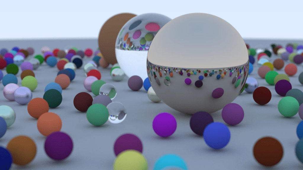
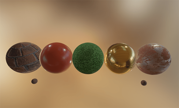


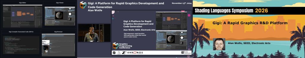


 to mean expected information entropy, but in other sources you’ll commonly see it as
  where
where  is the event, and
  are the outcomes.


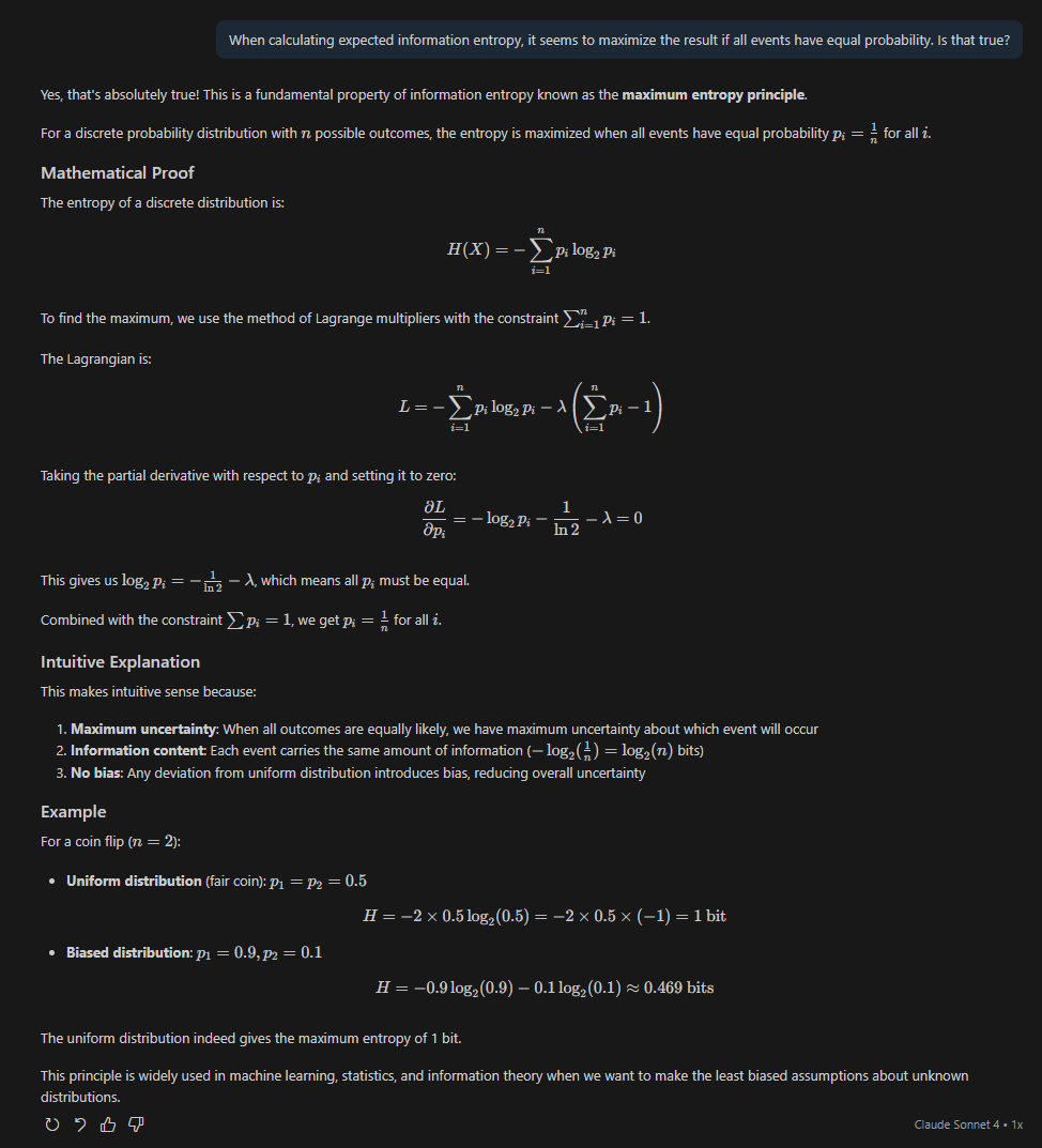


 , we can calculate the derivative as
  . Here are those two functions graphed.

 and wanted to know whether you should go left or right to get lower, the derivative can tell you. Plugging 1 into
  gives the value -4. A negative derivative means taking a step to the right will make the y value go down, so going right is down hill. We could take a step to the right and check the derivative again to see if we’ve walked far enough. As we are taking steps, if the derivative becomes positive, that means we went too far and need to turn around, and start going left. If we shrink our step size whenever we go too far in either direction, we can get arbitrarily close to the actual minimum point on the graph.
 and getting the value
  . Without iteration, we found that the minimum of the function is at
  term of a quadratic is negative, then it only has a maximum, instead of a minimum.
 that is a local minimum for x but a local maximum for y. The gradient will be zero in each direction, despite it not being a minimum, and the simulated ball will get stuck.
 , a gradient is a vector of derivatives, where you consider changing only one variable at a time, leaving the other variables constant. The notation for a gradient looks like this:
 , that means “The derivative of w with respect to x”. Another way of saying that is “If you added 1 to x before plugging it into the function, this is how much w would change, if the function was a straight line”. These are called partial derivatives, because they are derivatives of one variable, in a function that takes multiple variables.
 .
. .
. .
. .
. .
. .
.

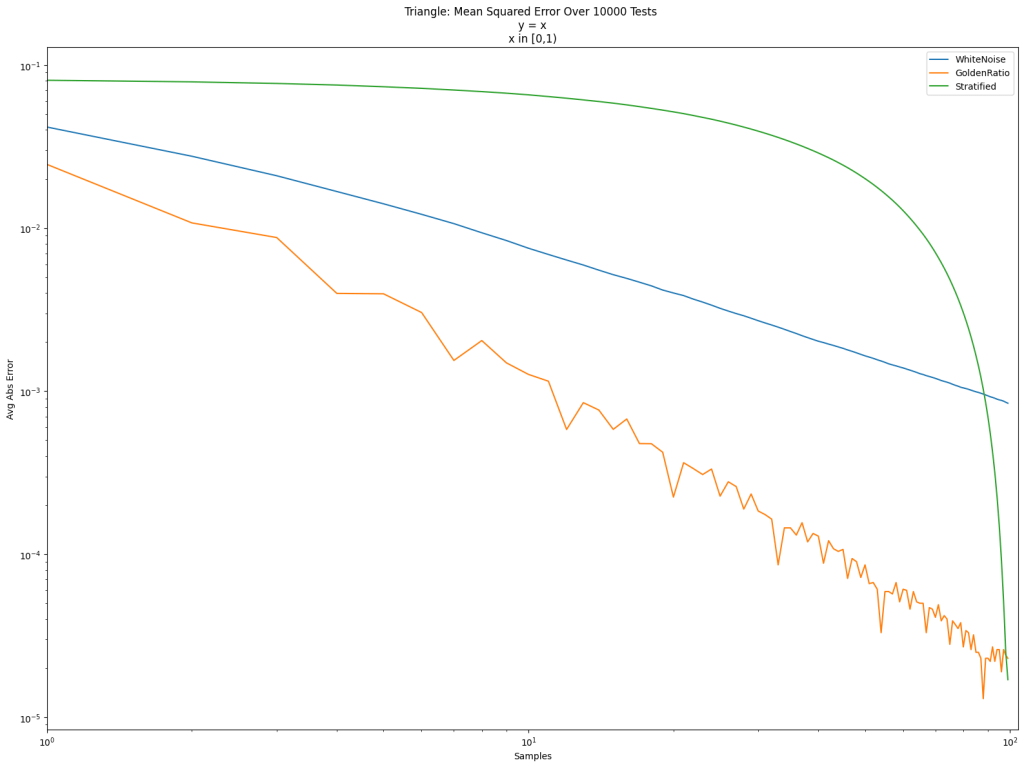

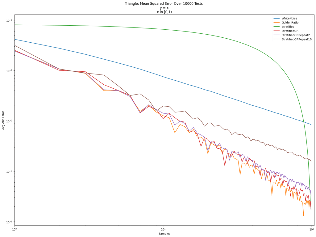
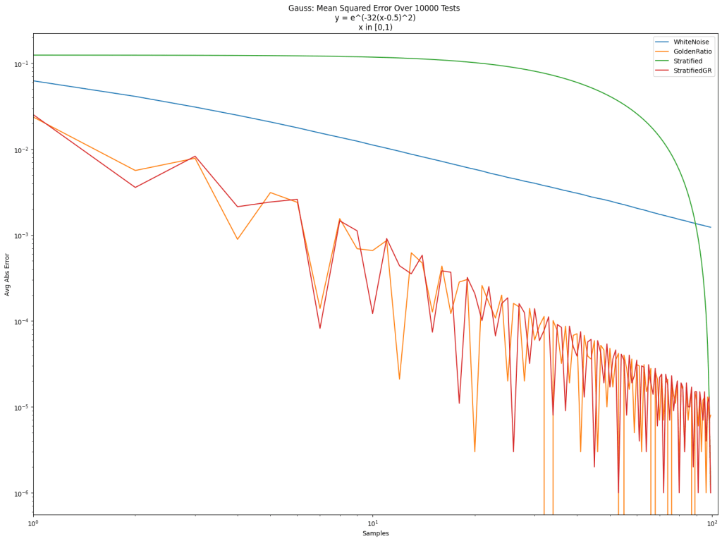
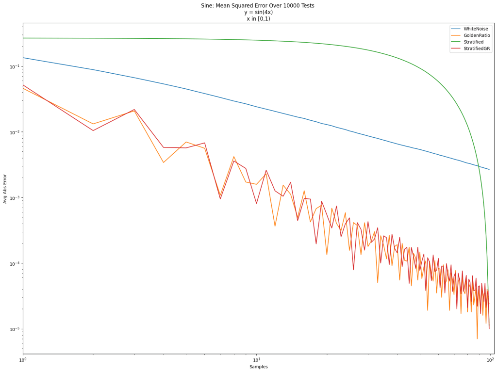
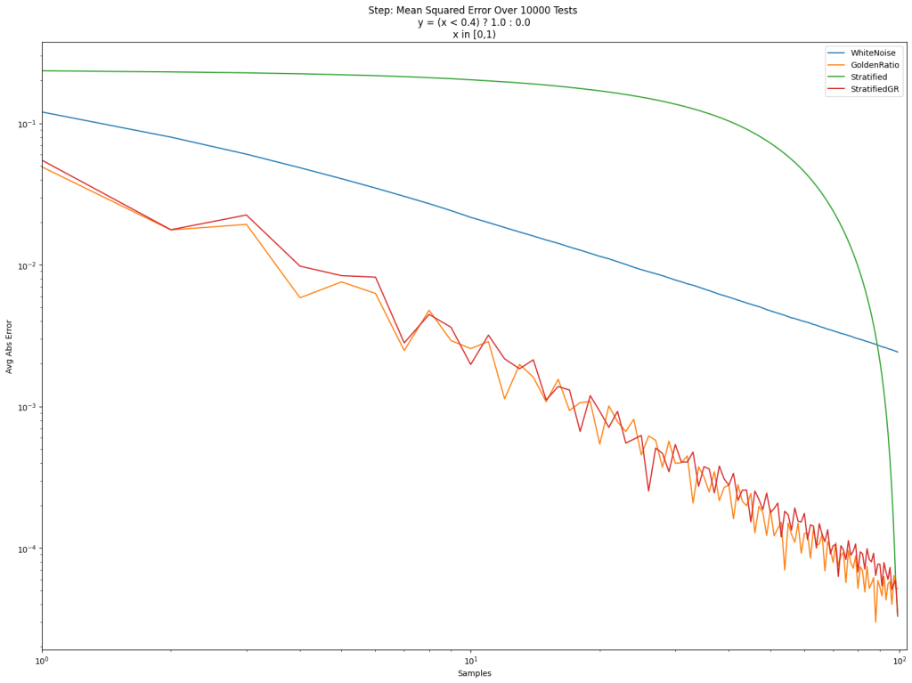
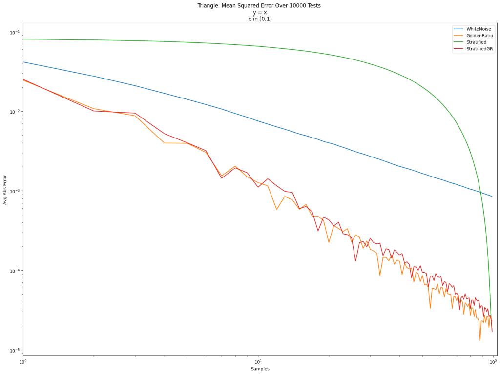


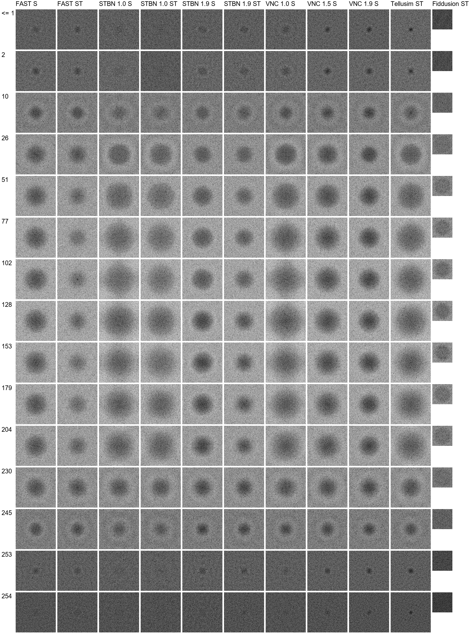


 . The value
  is what number is on the dice face, and the value
  says how many faces have that value.


 so that
  is 0.
is 0. because it makes all the
  power terms go away and leaves only the value of
  .
. because that will make all


 . The only way that can be true is if each dice has the
  . If we plug 1 in for


 , the
, the  which simplifies to:
 .
.


 can be true, when
 ![A,B,C \in [0,6]](https://s0.wp.com/latex.php?latex=A%2CB%2CC+%5Cin+%5B0%2C6%5D&bg=ffffff&fg=666666&s=0&c=20201002) .
. . If we want to do that three times – once for A, once for B, once for C – and add them together, we multiply that generating function by itself three times, aka we cube it.

 is 28, which means there are 28 different ways to add the three numbers between 0 and 6 together, to get 12.


 into infinity, but we know there are 20 jellybeans total, so we can stop at 20.