The 1990s! They felt like a wasteland of culture at the time, but looking back, there was hyper color t-shirts, the beginning of mainstream computing and the internet, the height of alternative rock, and of course magic eye pictures.
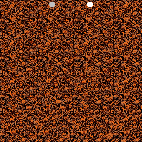
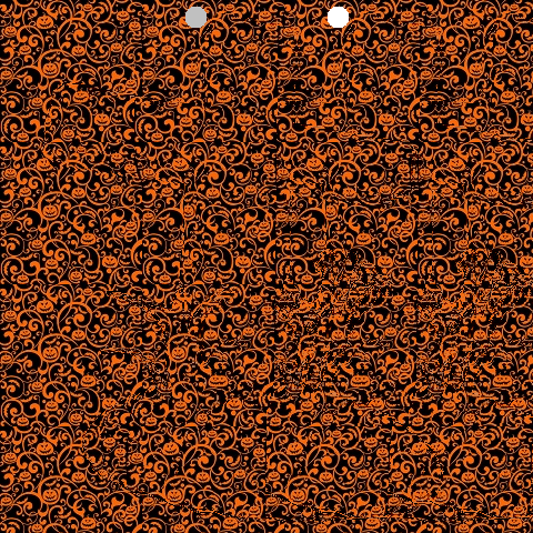
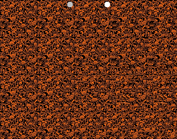
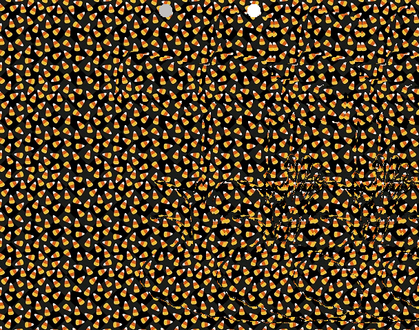
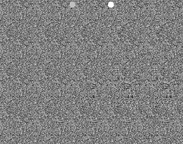
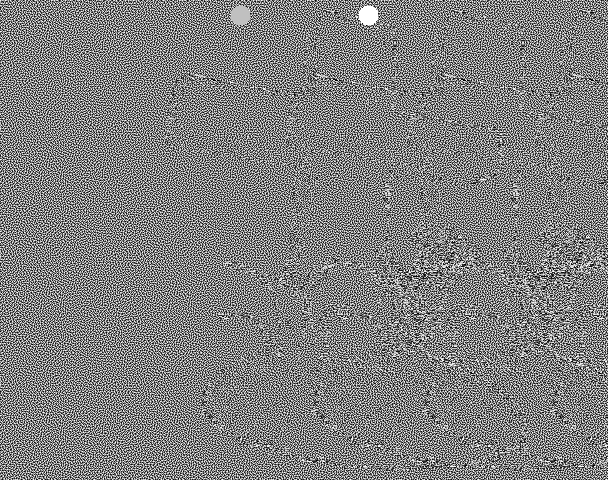
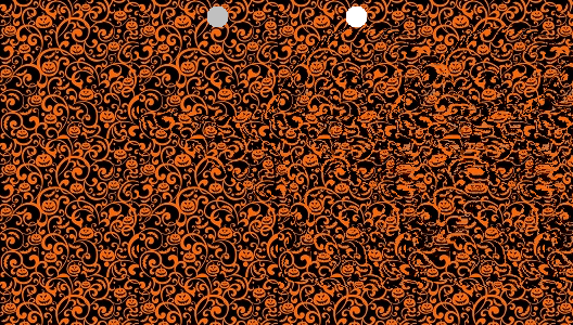
Unfocus your eyes such that the two dots overlap. A 3D image should emerge!
Quick PSA if you can’t see it!
To make an autostereogram, you need two things: 1. Color Image: A tileable repeating pattern. This can also just be “white noise”. 2. Depth Image: A grey scale depth map, or a black and white mask. This defines the 3D shape. Brighter pixel values are closer in depth.
For the above, I snagged these two from pintrest.
The image you are making is going to be the width and height of the depth image, but is going to have as many color channels as the color image.
You build the output image row by row, from left to right. To start out, we can just tile the output image with the color image. The Output Image pixel at (x,y) is the Color Image pixel at (x % ColorWidth, y % ColorHeight). That makes a tiled image, which does not have any 3d effect whatsoever:
To get a 3D effect we need to modify our algorithm. We need to read the Depth Image at pixel (x,y) to get a value from 0 to 255. We divide that by 255 to get a fractional value between 0 and 1. We then multiply that value by the “maximum offset amount”, which is a tuneable parameter (i set it to 20), to get an offset amount. This offset is how much we should move ahead in the pattern.
So, instead of Output Image pixel (x,y) using the Color Image pixel (x % ColorWidth, y % ColorHeight), we are calculating an offset from the Depth Image and using the Color Image pixel ((x + offset) % ColorWidth, y % ColorHeight).
Doing that, we aren’t quite there. Some 3D effects are starting to pop out, but it doesn’t look quite right.
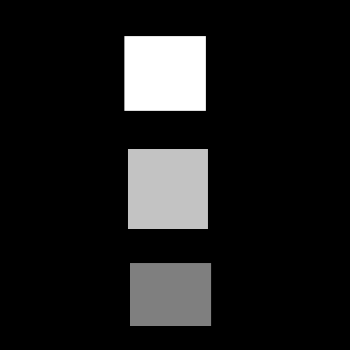
In fact, if you use the simpler depth map of the rectangles shown below, you can see the rectangles just fine, but there seems to be holes to the right of them.
What we need to do is not just look into the Color Image at an offset location, but that we need to look at the Output Image we are building, at an offset location. Specifically, we need to look at it in the previous color tile repetition. We use the Output Image pixel at ((x + offset – ColorWidth), y).
A problem with that though, is that when x is less than ColorWidth, we’ll be looking at a pixel x value that is less than 0 aka out of bounds. When x < ColorWidth, we should use the Color Image pixel instead, using the same formula we had before ((x + offset) % ColorWidth, y % ColorHeight).
That fixes our problem with the simpler squares depth map. The holes to the right are gone.
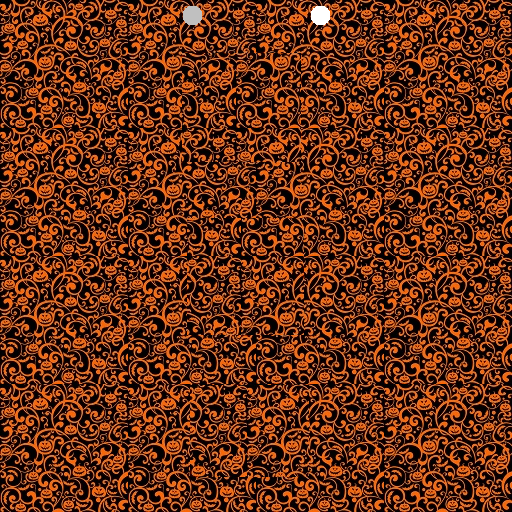
And it also mostly fixes our “grave” image:
There is one problem remaining with the grave image though. How these images work is that your left eye needs to lined up with an unmodified tile on the left, and your right eye needs to be lined up with a modified tile on the right. The grave image has depth information very close to the left side, which makes that not be possible. To fix this, you can add an extra “empty color tile” on the left. That makes our image a little bit wider but it makes it work. This also has the added benefit of centering the depth map, where it previously was shifted to the left a bit.
There we are, we are done!
Other Details
I found it useful to normalize the greyscale depth map. Some of them don’t use the full 0 to 1 range, which means they aren’t making the most use of the depth available. Remapping them to 0 to 1 helps that.
Some masks were meant to be binary black or white, but the images i downloaded form the internet had some grey in them (they were .jpg which is part of the problem – lossy compression). Having an option to binarize these masks was useful, forcing each pixel value or 0 or 1, whichever was closer.
The binary masks i downloaded had the part i was interested in being black, with a white background. I made the code able to invert this, so the interest part would pop out instead of receeding in.
The distance between the helper dots on the images are the width of the Color Image. A wider color image means a person has to work harder to get those dots to overlap, and it may not even be possible for some people (I’m unsure of details there hehe). I used tile sizes of 128.
It’s hard to make out fine detail from the depth maps. It seems like larger, coarse features are the way to go, instead of fine details.
More Pictures
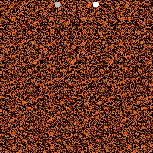
Here is the grave, with a different color texture. I find this one harder to see.
And another, using RGB white noise (random numbers). I can see this one pretty easily, but it isn’t as fun themed as the pumpkin image 🙂
And here is greyscale white noise (random numbers) used for the color image. I can see this just fine too.
I also tried using blue noise as a Color Image but I can’t see the 3d at all, and it isn’t a mystery what the 3d image is. You can see the repetition of the depth map object from the feedback. I think it’s interesting that the repetition is needed to make it look right. I have no understanding of why that is, but if you do, please leave a comment!
Here are some images that are not the grave. I find the pumpkin color texture works pretty nicely 🙂
Lastly, I think it would be really neat to make a game that used this technique to render 3d. It could be something simple like a brick breaking game, or as complex as a first person shooter. A challenge with this is that you need to process the image from left to right, due to the feedback loop needed. That won’t be the fastest operation on the GPU, forcing it to serialize pixel processing unless anyone has any clever ideas to help that. Still, it would be pretty neat as a tech demo!
This post is also about reducing the number of experiments needed, but uses orthogonal arrays, and is based on work by Genichi Taguchi (https://en.wikipedia.org/wiki/Genichi_Taguchi).
Let’s motivate this with a tangible situation. Imagine we are trying to find the best brownie recipe and we have three binary (yes/no) parameters. The first parameter “A” determines whether or not to add an extra egg. A value of 1 in a test means to add the egg, a value of 0 means don’t add the egg. The second parameter “B” determines whether to double the butter. The third option “C” determines whether we put nots on top.
Here are the 8 combinations of options, which you may recognize as counting to 7 in binary.
A (extra egg)
B (double butter)
C (add nuts)
Test 0
0
0
0
Test 1
0
0
1
Test 2
0
1
0
Test 3
0
1
1
Test 4
1
0
0
Test 5
1
0
1
Test 6
1
1
0
Test 7
1
1
1
Now we want to reduce the number of experiments down to 4, because we only have 4 brownie pans and also don’t want to get too fat trying to figure this out. Here are the 4 experiments we are going to do, along with a “result” column where we had our friends come over and rate the brownies from 1-10, and we took the average for each version of the recipe.
A
B
C
Result
Test 0
0
0
0
8
Test 1
0
1
1
6
Test 2
1
0
1
9
Test 3
1
1
0
7
At first glance the tests done seem arbitrary, and the results seem to not give us much information, but there is hidden structure here. Let’s highlight option A being false as bold, and true as being left alone.
A
B
C
Result
Test 0
0
0
0
8
Test 1
0
1
1
6
Test 2
1
0
1
9
Test 3
1
1
0
7
If you notice, we are doing two tests for A being false, and in those two tests, we have a version where B is true, and a version where B is false. The same is true for C; it’s true in one test and false in the other. This essentially makes the effects of the B and C options cancel out in these two tests, if we average the results.
Looking at the two tests for when A is true, the same thing happens. One test has B being true, the other false. One test has C being true, the other false. Once again this makes the effects of B and C cancel out, if we average the results.
Averaging the results when A is false gives us 7. Averaging the results when A is true gives us 8. This seems to indicate that adding an extra egg gives a small boost to the tastiness of our brownies. In our tests, due to the effects of B and C canceling out, we can be more confident that we really are seeing the results of the primary effect “A” (Adding an extra egg), and not some secondary or tertiary effect.
More amazingly, we can highlight the tests where B is false and see that once again, in the two tests for B being false, A and C have both possible values represented, and cancel out again. Same for when B is true.
A
B
C
Result
Test 0
0
0
0
8
Test 1
0
1
1
6
Test 2
1
0
1
9
Test 3
1
1
0
7
The same is true if we were to highlight where C is false. Every parameter is “isolated” from the others by having this property where the other parameters cancel out in the tests.
Let’s make a table showing the average scores for when A,B and C are false vs true.
No
Yes
A (extra egg)
7
8
B (double butter)
6.5
8.5
C (nuts on top)
7.5
7.5
From this table we can see that doubling the butter gives the biggest increase in score to our brownies. Adding another egg helps, but not as much. Lastly, people don’t seem to care whether there are nuts on top of the brownies or not.
It’s pretty neat that we were able to do this analysis and make these conclusions by only testing 4 out of the 8 possibilities, but we also have missing information still – what we called aliases in the last blog post. Software that deals with fractional factorial experiment design (there’s one called minitab) are able to show the aliasing structure of these “Taguchi Orthogonal Arrays”, but I wasn’t able to find how to calculate what the aliases are exactly. If someone figures that out, leave a comment!
I just spilled the beans, in that the table of tests to do is called an “Orthogonal Array”. More specifically it’s an orthogonal array of strength 2.
For an orthogonal array of strength 2, you can take any 2 columns, and find all possible combinations of the parameter values an equal number of times. Here is the testing table again, along with the values of “AB”, “AC”, and “BC” to show how they each have all possible values (00, 01, 10, 11) exactly once.
A
B
C
AB
AC
BC
Test 0
0
0
0
00
00
00
Test 1
0
1
1
01
01
11
Test 2
1
0
1
10
11
01
Test 3
1
1
0
11
10
10
Orthogonal arrays give this isolation / cancellation property that allows you to do a reduced number of tests, and still make well founded conclusions from the results.
A higher strength orthogonal array means that a larger number of columns can be taken, and the same will be true. This table isn’t a strength 3 orthogonal array, because it is missing some values. The full factorial test on these three binary parameters would be a strength 3 orthogonal array, which gives better results, but is full factorial, so doesn’t save us any time.
Unlike the last blog post, parameters don’t have to be limited to binary (2 level) values with these arrays. We could turn parameter A (add an extra egg) into something that had three values: 0 = regular amount of eggs, 1 = an extra egg, 2 = two extra eggs.
The full factorial number of tests would then become 12 instead of 8:
A (3 level)
B (2 level)
C (2 level)
Test 0
0
0
0
Test 1
0
0
1
Test 2
0
1
0
Test 3
0
1
1
Test 4
1
0
0
Test 5
1
0
1
Test 6
1
1
0
Test 7
1
1
1
Test 8
2
0
0
Test 9
2
0
1
Test 10
2
1
0
Test 11
2
1
1
Unfortunately in this case, there is no strength 2 orthogonal array that is smaller than the full 12 tests. The reason for this is because an orthogonal array needs pairs of columns to have an equal number of each possible value, for that pairs of columns. The column pairs of AB and AC both have 6 values, while the column pair BC has 4 values. If we did only 4 tests, the AB and AC column pairs would be missing 2 out of the 6 possible values. If we did 6 tests, the column pair BC would have 2 extra values, which can also be seen as missing 2 values to make it have all values twice.
To formalize this, the minimum number of tests you can do is the least common multiple of the column pair value combinations. In this example again, AB and AC have 6, while BC has 4. The least common multiple between 6 and 4 is 12. So, you need to do a multiple of 12 experiments with this setup to make an orthogonal array. The full factorial array is size 12, and in fact is the orthogonal array that we are talking about.
If you add another 2 level factor (binary parameter), the minimum number of experiments stays at 12, but the full factorial becomes 24, so we are able to beat the full factorial in that case.
A (3 level)
B (2 level)
C (2 level)
D (2 level)
Test 0
0
0
0
1
Test 1
0
0
1
0
Test 2
0
1
0
1
Test 3
0
1
1
0
Test 4
1
0
0
1
Test 5
1
0
1
0
Test 6
1
1
0
0
Test 7
1
1
1
1
Test 8
2
0
0
0
Test 9
2
0
1
1
Test 10
2
1
0
0
Test 11
2
1
1
1
Robustness Against Uncontrolled Variables
I’ve only read a little about Taguchi but what I have read has really impressed me. One thing that really stood out to me is nearly a social issue. Taguchi believed making precise results was the correct ultimate goal of a factory. He believed erratic and low quality results affected the consumer and the company, and demonstrated how both ultimately affected the company. From wikipedia:
Taguchi has made a very influential contribution to industrial statistics. Key elements of his quality philosophy include the following:
Taguchi loss function, used to measure financial loss to society resulting from poor quality;
The philosophy of off-line quality control, designing products and processes so that they are insensitive (“robust”) to parameters outside the design engineer’s control.
Innovations in the statistical design of experiments, notably the use of an outer array for factors that are uncontrollable in real life, but are systematically varied in the experiment.
I’d like to highlight his work in making processes robust against uncontrolled variables.
What you do is run the tests when the uncontrolled variable is a certain way, then when it’s another way, you run the tests again. You might do this several times.
Then, for each combination of settings you do have control over, you take the standard deviation for when the uncontrolled variable varies. Whichever combination of controllable settings gives you the lowest standard deviation (square root of variance), means that setting of variables is least affected by the uncontrolled variable.
It may not be the BEST result, but it lets you have a CONSISTENT result, in uncontrollable conditions. Sometimes consistency is more important than getting the best score possible. FPS in a video game is an example of this. A smooth frame rate feels and appears a lot better perceptually than a faster, but erratic frame rate.
Note that you can use this technique with CONTROLLABLE variables too, to see if there are any variables that don’t have a strong impact on the result. You can use this knowledge to your advantage by removing it from future tests as a variable for example.
Here is another example of where that could be useful. Imagine you were making a video game, and you provided the end user with a set of graphics options to help them control the game’s performance on their machine. If you run tests of different performance, for different graphics settings, on different machines, you might find that certain settings don’t help performance much AT ALL for your specific game. If this is the case, you can remove the graphics setting from the UI, and set it to a constant value. Simplifying the settings helps you the developer, by having fewer code paths to maintain, it helps QA by having fewer code paths to test, and it helps the user, by only presenting meaningful graphics options.
An Algorithm For Orthogonal Array Generation
I couldn’t find a singular orthogonal array generation algorithm on the net. From what I read, there are different ways of constructing different types of orthogonal arrays, but no generalized one. However, it’s easy enough to craft a “greedy algorithm with backtracking” algorithm, and I did just that. The source code can be found at https://github.com/Atrix256/OrthogonalArray.
Let’s think of the orthogonal array as a matrix where each row is an experiment, and each column lists the values for a parameter across all of the experiments. The goal we are after is to have each column pair have each possible value show up once.
Assuming that all columns have the same number of possible values for a moment (like, they are all binary and can either have a 0 or 1), we can see that when filling up any single column pair with options, we will also fill up all of the other column pairs. As a concrete example, if we have 3 binary columns A,B,C, we know that by filling AB with all the values 00, 01, 10, 11 by choosing experiments from the “full factorial list”, that there will also be four values in the columns AC and BC. So, we only need to find 4 rows (specific experiments) in that case. We can just fill up the first column pair, and the other column pairs will get filled up too.
We can do this by choosing any experiment that has 00 in AB, then 01, 10, and finally 11.
However, the values that fill up the other columns may not end up in the full set of values, and there may be repeats, even if we disallow repeats of specific experiments.. Column AC may end up being 00, 00, 11, 10 for instance which has 00 showing up twice, and 01 doesn’t show up at all.
So, when we choose an experiment (row) to use that matches the value we want from the AB column, we also have to make sure it isn’t a duplicate value in any of the other columns.
Doing this, we may end up in a spot where we have values left to fill in, but none of our options are valid. At this point, we take a step back, remove the last row we added, and try a new one. This is the backtracking. We may have to backtrack several steps before we find the right solution. We may also exhaustively try all solutions and find no solution at all!
Generalizing this further, our columns may not all have the same number of possible values – like in our examples where we mixed 3 level and 2 level variables. As I mentioned before, some column pairs will have 6 possible values, while others will have 4 possible values. The only way you can make an orthogonal array in that situation is by making a number of rows that are a multiple of the least common multiple of 6 and 4, which is 12. The 6 value column pairs will have all values twice, and the 4 value column pairs will have each value three times.
Lastly, there are situations where no solution can be found by repeating the values this minimal number of times, but if you do twice as many (or more), a solution can be found, and still be smaller than the full factorial set of experiments. An example of this is if you have five 3 level factors. You cant make an orthogonal array that is only 9 rows long, but you can make one that is 18 rows long. That is still a lot smaller than the full factorial number of experiments which is 3^5 or 243 experiments.
Closing and Links
From the number of reads of the previous blog post, this seems to be a topic that really resonates with people. Who doesn’t want to do less work and still get great results? (Tangent: That is also the main value of blue noise in real time rendering!)
In these two posts, we’ve only scratched the surface. Apparently there is still researching coming out about this family of techniques – doing a smaller number of tests and gleaming the most relevant data you can from them.
When starting on this journey, I thought it must surely have applications to sampling in monte carlo integration, and indeed it does! There is a paper from 2019 i saw, but didn’t understand at the time, which uses orthogonal arrays for sampling (https://cs.dartmouth.edu/~wjarosz/publications/jarosz19orthogonal.html).
The rabbit hole has become quite deep, so I think I’m going to stop here for now. If you have more to contribute here, please leave a comment! Thanks for reading!
Have you ever found yourself in a situation where you had a bunch of parameters to tune for a better result, but there were just too many to exhaustively search all possibilities?
I recently saw a video that talked about how to reduce the number of experiments in these situations, such that it formalizes what conclusions you can and cannot make from those experiments. Even better, the number of experiments can be a sliding scale to either be fewer experiments (faster), or more information from the results (higher quality).
We are going to explore a method for doing that in this post, but you should also give the video a watch before or after reading, as it talks about a different method than we will! https://www.youtube.com/watch?v=5oULEuOoRd0
Fractional Factorial Design Terminology
The term “fractional factorial” is in contrast to the term “full factorial”.
To have some solid context, let’s pretend that we want to figure out how to make the best brownies, and we have 3 options A, B, C. Option “A” may be “add an extra egg”, “B” may be “double the butter” and “C” may be “put nuts on top”, where 1 means do it, and -1 means don’t do it.
Three parameters with two choices each means we have 8 possibilities total:
A
B
C
Test 0
-1
-1
-1
Test 1
-1
-1
1
Test 2
-1
1
-1
Test 3
-1
1
1
Test 4
1
-1
-1
Test 5
1
-1
1
Test 6
1
1
-1
Test 7
1
1
1
We’ve essentially counted in binary, doing all 8 tests for all 8 possibilities of the three binary parameters.
If you’ve noticed that the number of tests are 2^3, and not a factorial, you are correct. The term “factorial” refers to “factors” which is another name for a parameter. We have 3 factors in our experiment to make the best brownies.
Each factor has two possible values. In the literature, the number of values a parameter can take is called a level. So, our brownie experiment has 3 two level factors.
If we didn’t have enough pans to bake all 8 types of brownies, we may instead opt to do a smaller amount. We may only do 1/2 of the tests for instance, which means that we would be doing a fractional amount of the full factorial experiment. We’d be doing a fractional factorial experiment. We could even do 1/4 of the experiments. The fewer experiments we do, the less information we get.
Choosing which four experiments to do, and knowing what conclusions we can draw form the results is where the magic happens.
Fractional Factorial Design
Going back to our brownie recipe, let’s say that we want to do 4 bakes, instead of 8.
We start by making a full experiment table for A and B, but leave C blank
A
B
C
Test 0
-1
-1
Test 1
-1
1
Test 2
1
-1
Test 3
1
1
We now have to decide on a formula for how to set C’s value, based on the value of A and B. This is called a generator and to test things out, lets set C to the same value as A, so our generator for C is “C = A”
A
B
C=A
Test 0
-1
-1
-1
Test 1
-1
1
-1
Test 2
1
-1
1
Test 3
1
1
1
We have 4 experiments to do now, instead of 8, but it isn’t obvious what information we can get from the results. Luckily some algebra can help us sort that out. This algebra is a bit weird in that any letter squared becomes “I”, or identity. Our ultimate goal is to find the “Aliasing Structure” of our experiments, which is made up of “words”. Words are combinations of the parameter letters, as well as identity “I”. The aliasing structure lets you use algebra to find what testing parameters alias with other testing parameters. An alias means you can’t tell one from the other, with the limited number of tests you’ve done.
That is quite a lot of explaining, so lets actually do these things.
First up we have C = A. If we multiply both sides by C we get CC = AC. Any value multiplied by itself is identity, so we get I = AC as a result. Believe it or not, that is our full aliasing structure and we are done! We’ll have more complex aliasing structures later but we can keep it simple for now.
Now that we have our aliasing structure, if we want to know what something is aliased by, we just multiply both sides by our query to get the result. Here’s a table to show what I mean.
Alias Query
Result
I
I = AC
A
A = AAC = C
B
B = ABC
C
C = ACC = A
AB
AB = AABC = BC
AC
AC = AACC = I
BC
BC = ABCC = AB
ABC
ABC = AABCC = B
Looking at the table above, we see that B = ABC. This means that B aliases ABC. More plainly, this means that from our experiments, if the brownies were rated from 1 to 10 for tastyness, we wouldn’t be able to tell the difference in results between only doing option B (doubling the butter) and doing all three options: adding an egg, doubling the butter, and adding nuts on top.
Another thing we can see in the table is that A = C. That means that we cannot tell the difference between adding an egg, or adding nuts on top.
Lastly, I = AC means that we can’t tell the difference between doing nothing at all, compared to adding an egg and adding nuts on top.
If we care to be able to distinguish any of these things, we’d have to change our experiment design. Specifically, we would need to change the generator for C.
We can do that, and in fact there is a better choice for a generator for C. Let’s make it so that value of C is the value of A and B multiplied together. C = AB.
A
B
C=AB
Test 0
-1
-1
1
Test 1
-1
1
-1
Test 2
1
-1
-1
Test 3
1
1
1
It doesn’t look like much has changed, but lets do the same analysis as before.
We can get our aliasing structure by starting with C=AB and multiplying both sides by C to get CC=ABC, which simplifies to I = ABC. Let’s find all of our aliases again.
Alias Query
Result
I
I = ABC
A
A = BC
B
B = AC
C
C = AB
AB
AB = C
AC
AC = B
BC
BC = A
ABC
ABC = I
Something interesting has happened with this design of experiments (D.O.E.). All of the single letters alias with double letters. This means that we can distinguish all primary effects from each other, but that primary effects are aliased (or get “confounded”) with secondary effects. In many situations, the primary effects are more prominent than secondary effects (adding butter or adding nuts is more impactful individually, than when combined). In these situations, you can assume that if there’s a big difference noticed, that it is the primary effect causing it. If there’s any doubt, you can also do more focused experiment(s) to make sure your assumptions are correct.
Resolution
So why is it that our first generator C=A wasn’t able to differentiate primary effects, while our second generator C=AB could? For such a simple example, it might be obvious when looking at C=A, but this has to do with something called “Resolution”, which is equal to the length of shortest word in the aliasing structure (not counting I).
With I=CA, that is two letters, so it is a resolution II D.O.E. Resolution II D.O.E.s have at least some primary effects aliased (or confounded) with other primary effects. Resolution II D.O.E.s are usually not very useful.
With I=ABC, that is three letters, so is a resolution III D.O.E. Resolution III D.O.E.s have primary effects aliased with secondary effects. These are more useful, as we explained above.
As you add more factors, you can get even higher resolution D.O.E.s. A resolution IV has primary effects aliased with tertiary effects, and secondary effects are aliased with each other. A resolution V has primary effects aliased with quaternary effects, and secondary effects are aliased with tertiary effects. If you are noticing the pattern that the aliasing effect classes add up to the resolution, you are correct, and that pattern holds for all resolutions.
Getting a higher resolution D.O.E. is usually better, so you want your generators to contain more letters. You have to be careful to make them unique enough though. If you had four factors A,B,C,D and generators C=AB, D=AB, you can see that you’ve introduced an alias C=D.
If you work out the aliasing structure, this problem becomes apparent that you’ve made a resolution II D.O.E. Aliasing structures always need 2^p words, where p is the number of parameters that have generators. In this case, p is 2, so you need 2^2 or 4 words in the aliasing structure.
The first word comes from C=AB, which can be rewritten as I=ABC. Actually that’s the first two words.
The second word comes from D=AB, which can be rewritten as I=ABD. That gives us three words:
I = ABC = ABD
To get the fourth word, we can see that both ABC and ABD are equal to each other. Remembering that when we multiply the same thing against itself we get identity, we can make our fourth word by multiplying them together to get something equal to identity for our aliasing structure.
ABC*ABD = AABBCD = CD.
So, our four words all together are:
I = ABC = ABD = CD
Since “CD” is the shortest word that is not identity, and is 2 letters, we can conclude that we have a resolution II D.O.E.
We can multiply the aliasing structure by C to get all the things that C is aliased with.
C = AB = ABCD = D
This shows we cannot tell the difference between C and D, because they are aliased, or confounded, and confirms that we have a resolution II D.O.E.
What’s With The Weird Algebra?
When we said C=AB, where A and B were either -1 or +1 in each column, it was pretty easy to just multiply the values together to get the result.
What probably made less sense is when working with the generators and aliasing structures, why a letter times itself would become identity. The reason for this is that the multiplication is a component wise vector product. If the original value was -1, then we get -1*-1 or +1. If the original value was +1, then we get 1*1 or +1. The result of a component wise vector product between a vector and itself will have a 1 in every component, which is identity.
To help cement these ideas, we’ll do one more example with 8 experiment and 5 factors. That means we’ll only do 1/4 of the experiments we would if doing the full factorial, doing 8 experiments instead of 32.
8 experiments mean that the first three factors will be full factorial, and the last two parameters will need generators. We’ll use D = AB and E=BC as our generators.
We can make our experiment table to start.
A
B
C
D=AB
E=BC
Test 0
-1
-1
-1
1
1
Test 1
-1
-1
1
1
-1
Test 2
-1
1
-1
-1
-1
Test 3
-1
1
1
-1
1
Test 4
1
-1
-1
-1
1
Test 5
1
-1
1
-1
-1
Test 6
1
1
-1
1
-1
Test 7
1
1
1
1
1
Let’s also make our aliasing structure. Since we are using generators on 2 parameters, that means p=2, and so we have 2^p = 2^2 = 4 words in our aliasing structure. The first 3 are easy, since they come from our generators directly.
D = AB : I = ABD E = BC : I = BCE so: I = ABD = BCE
For the fourth word, we again know that ABD and BCE are equal since they are both equal to identity. We also know that multiplying anything by itself is identity, so we can multiply them together to get the fourth word:
ABD*BCE = ABBCDE = ACDE
Our full aliasing structure is then the below, which shows that we have a resolution III D.O.E, meaning primary effects are only aliased with secondary effects.
I = ABD = BCE = ACDE
Lastly, let’s make the full 32 entry table showing all aliases to understand the things we can, and cannot differentiate from our experiment results.
Alias Query
Result
I
I = ABD = BCE = ACDE
A
A = BD = ABCE = CDE
B
B = AD = CE = ABCDE
C
C = ABCD = BE = ADE
D
D = AB = BCDE = ACE
E
E = ABDE = BC = ACD
AB
AB = D = ACE = BCDE
AC
AC = BCD = ABE = DE
AD
AD = B = ABCDE = CE
AE
AE = BDE = ABC = CD
BC
BC = ACD = E = ABDE
BD
BD = A = CDE = ABCE
BE
BE = ADE = C = ABCD
CD
CD = ABC = BDE = AE
CE
CE = ABCDE = B = AD
DE
DE = ABE = BCD = AC
ABC
ABC = CD = AE = BDE
ABD
ABD = I = ACDE = BCE
ABE
ABE = DE = AC = BCD
ACD
ACD = BC = ABDE = E
ACE
ACE = BCDE = AB = D
ADE
ADE = BE = ABCD = C
BCD
BCD = AC = DE = ABE
BCE
BCE = ACDE = I = ABD
BDE
BDE = AE = CD = ABC
CDE
CDE = ABCE = BD = A
ABCD
ABCD = C = ADE = BE
ABCE
ABCE = CDE = A = BDE
ABDE
ABDE = E = ACD = BC
ACDE
ACDE = BCE = ABD = I
BCDE
BCDE = ACE = D = AB
ABCDE
ABCDE = CE = AD = B
Closing
A limitation you may have noticed in this article is that it only works with binary parameters (2 level factors). Part 2 of this blog post will show how to overcome that limitation using a different technique for fractional factorial experimental design.
Until then, there is a way to extend this method to factors which have a multiple of 4 levels. If you are interested in that, google Plackett-Burman.