I haven’t made many blog posts this year, due to working on a project at work that I just got open sourced. The project is called Gigi and it is a rapid prototyping and development platform for real time rendering, and GPU programming. We’ve used it to prototype techniques and collaborate with game teams, we’ve used it in published research (FAST noise), and used it to generate code we’ve shared out into the world.

More info on Gigi is here: https://github.com/electronicarts/gigi/

I also used Gigi to do the experiments and make the code that go with this blog post. Both the Gigi source files and the C++ DX12 code generated from those Gigi files are on github at https://github.com/Atrix256/BNOctaves.

Motivation

Link: https://mastodon.gamedev.place/@lisyarus/113057251773324600

Nikita tagged me in this interesting post with a neat looking screenshot. I thought this was interesting and wanted to look deeper so got the details.

The idea is that you start with a blue noise texture. You then add in another blue noise texture, but 2x bigger and multiplied by 1/2. You then add in another blue noise texture again, but 4x bigger, and multiplied by 1/4. Repeat this as many times as desired. While doing this process you sum up the weights (1 + 1/2 + 1/4 + …) and you divide the result by the weight to normalize it.

Results – Blue Noise

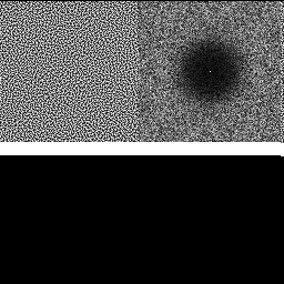
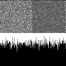
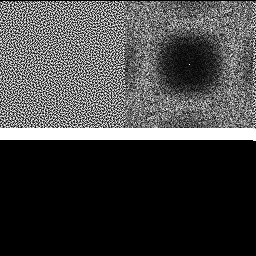
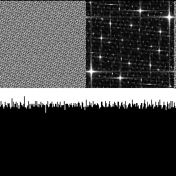
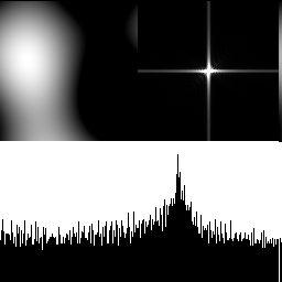
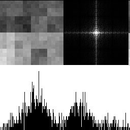
Here is a blue noise texture by itself, made using the FAST command line utility (https://github.com/electronicarts/fastnoise). The upper left is the noise texture. The upper right is the DFT to show frequency content, and the bottom half is a histogram. Here we can see that the texture is uniform blue noise. The histogram shows the uniform distribution, and the DFT shows that the noise is blue, because there is a dark circle in the center, showing that the noise has attenuated low frequencies.

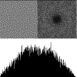
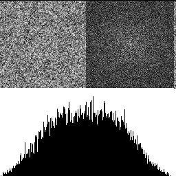
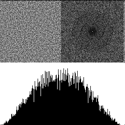
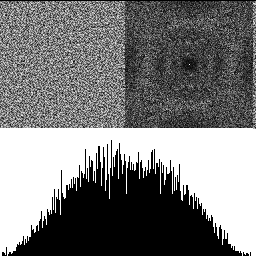
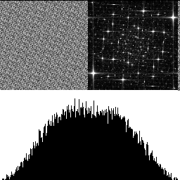
With 2 octaves shown below, there are lower frequencies present, and the histogram gets a hump in the middle. The low frequencies increase because when we double the size of the texture, it lowers the frequency content. The reason the histogram is no longer uniform is because of the central limit theorem. Adding random numbers together makes them follow a binomial distribution, and Gaussian at the limit (more info: https://blog.demofox.org/2019/07/30/dice-distributions-noise-colors/).

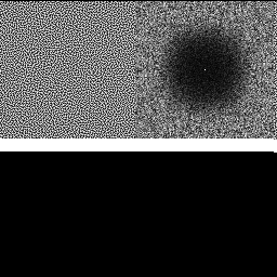
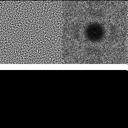
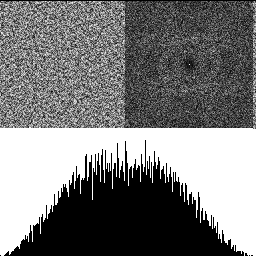
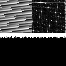
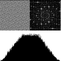
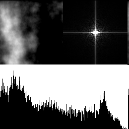
With 3 octaves shown below, the effects are even more pronounced.

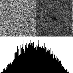
So yeah, adding octaves of blue noise together does produce blue noise! It makes the distribution more Gaussian though, and reduces the frequency cutoff of the blue noise.

Note: It doesn’t seem to matter much if I use the same blue noise texture for each octave, or different ones. You can control this in the demo using the “DifferentNoisePerOctave” checkbox.

Results – Other Noise Types

After going through the work of making this thing, I wanted to see what happened using different noise types too.

White Noise

Here is 1 octave of white noise, then 3 octaves. White noise starts with randomized but roughly equal levels of noise in each frequency. This process looks to make the low frequencies more pronounced, which makes sense since the octaves get bigger and so are lower frequency.

3×3 Binomial Noise

This noise type is something we found to rival “traditional” (gaussian) blue noise while writing the FAST paper. Some intuition here is that while blue noise has a frequency cutoff equal distance from the center (0hz aka DC), this binomial noise frequency cutoff has roughly equal distance from the edges (aka nyquist). More info on FAST here https://www.ea.com/seed/news/spatio-temporal-sampling.

Below is 1 octave, then 3 octaves. It seems to tell the same story, but the 3 octaves seem to have some concentric rings in the DFT which is interesting.

3×3 Box Noise

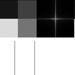
Here is noise optimized to be filtered away using a 3×3 box filter. 1 octave, then 3 octaves.

5×5 Box Noise

Here is noise optimized to be filtered away using a 5×5 box filter. 1 octave, then 3 octaves.

Results – Low Discrepancy Noise Types

Here are some types of low discrepancy noise.

Interleaved Gradient Noise

Interleaved gradient noise is a low discrepancy object that doesn’t really have a name in formal literature. I call it a low discrepancy grid, which means we can use it as a per pixel source of random numbers, but it has low discrepancy properties spatially. It was invented by Jorge Jimenez at Activision and you can read more about it at https://blog.demofox.org/2022/01/01/interleaved-gradient-noise-a-different-kind-of-low-discrepancy-sequence/.

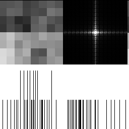
Here is 1 octave then 3 octaves. The DFT goes from a starfield to a more dense starfield.

R2 Noise

R2 is a low discrepancy sampling sequence based on the golden ratio (https://extremelearning.com.au/unreasonable-effectiveness-of-quasirandom-sequences/), but you can also turn it into a “low discrepancy grid”. You do so like this:

// R2 Low discrepancy grid
// A generalization of the golden ratio to 2D
// From https://extremelearning.com.au/unreasonable-effectiveness-of-quasirandom-sequences/
float R2LDG(uint2 pos)
{
	static const float g  = 1.32471795724474602596f;
	static const float a1 = 1 / g;
	static const float a2 = 1 / (g * g);
	return frac(float(pos.x) * a1 + float(pos.y) * a2);
}

1 octave, then 3 octaves. The DFT goes from a starfield, to a swirly galaxy. That is pretty cool honestly! The histogram also have a lot less variance than other noise types, which is a cool property.

Wait… Isn’t This Backwards?

When we make Perlin noise, we start with the chunky noise first at full weight, then we add finer detail noise at less weight, like the below with 1 and 8 octaves of perlin noise.

In our noise experiments so far, we’ve been doing it backwards – starting with the smallest detailed noise at full weight, then adding in chunkier noise as lower weight. What if we did it the other way? The demo has a “BlueReverse” noise type that lets you look at this with blue noise. Here is 1, 3 and 5 octaves:

It has an interesting look, but does not result in blue noise!

Use of Gigi – The Editor

I used Gigi to make the demo and do the experiments for this blog post. You can run the demo in the Gigi viewer, or you can run the C++ dx12 code that Gigi generated from the technique I authored.

I want to walk you through how Gigi was used.

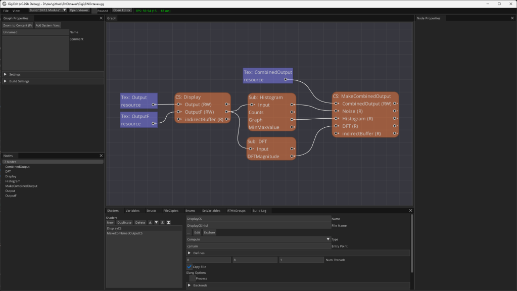
Below is the technique in the Gigi editor. The “CS: Display” node makes the noise texture with the desired number of octaves. “Sub: Histogram” makes the histogram graph. “Sub: DFT” makes the DFT. “CS: MakeCombinedOutput” puts the 3 things together into the final images I pasted into this blog post.

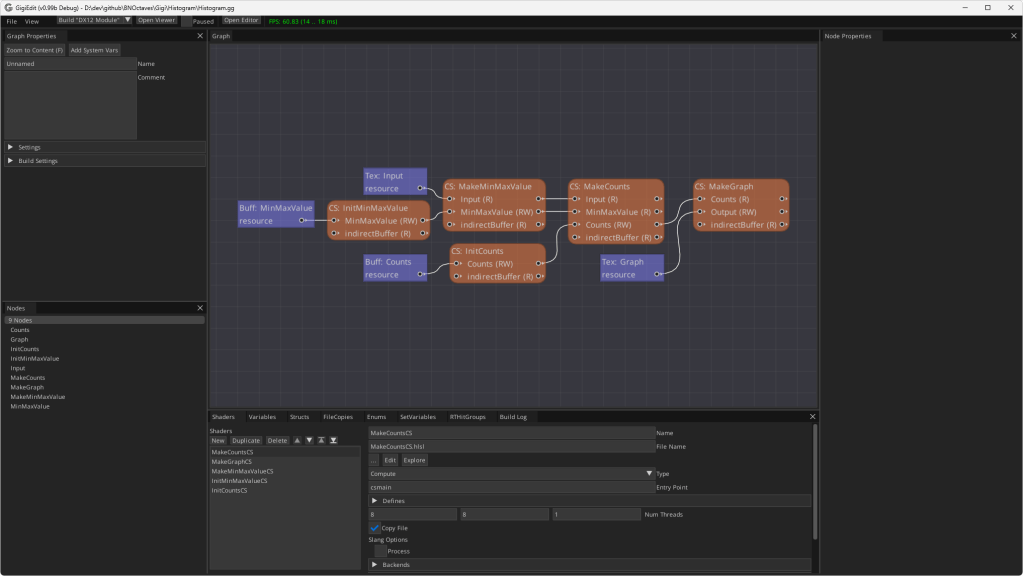
If you double click the “Sub: Histogram” subgraph node, it shows you the process for making a histogram for whatever input texture you give it. This is a modular technique that you could grab and use in any of your Gigi projects, like it was used here!

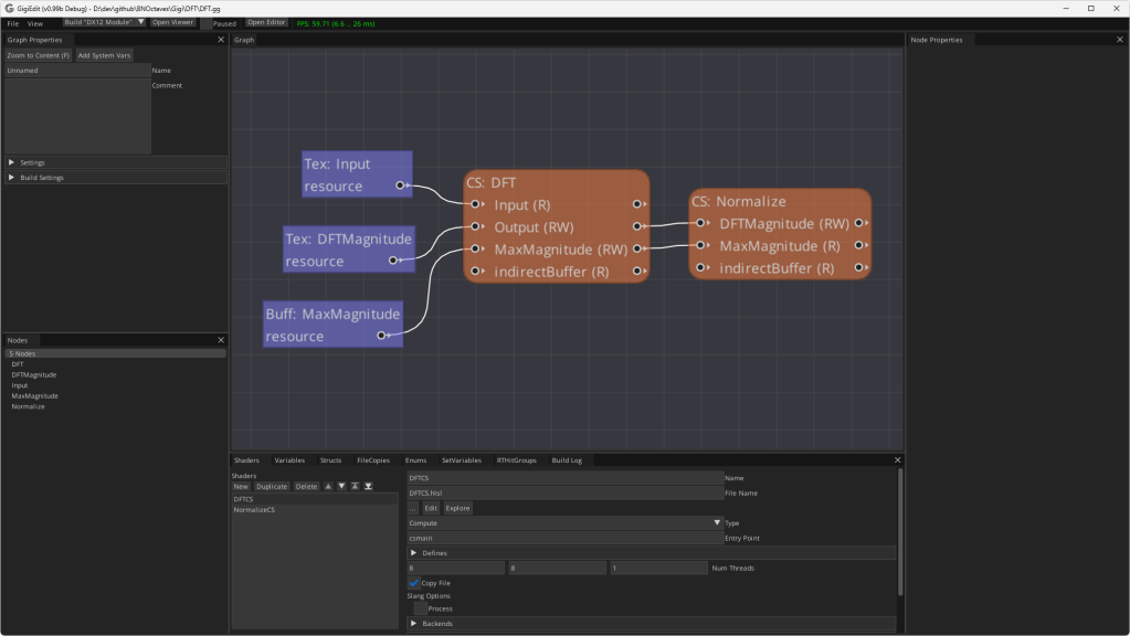
If you double click the “Sub: DFT” subgraph node instead, you would see this, which is also a modular, re-usable technique if ever you want to see the frequency magnitudes of an image. Note: This DFT is not an FFT, it’s a naive calculation so is quite slow.

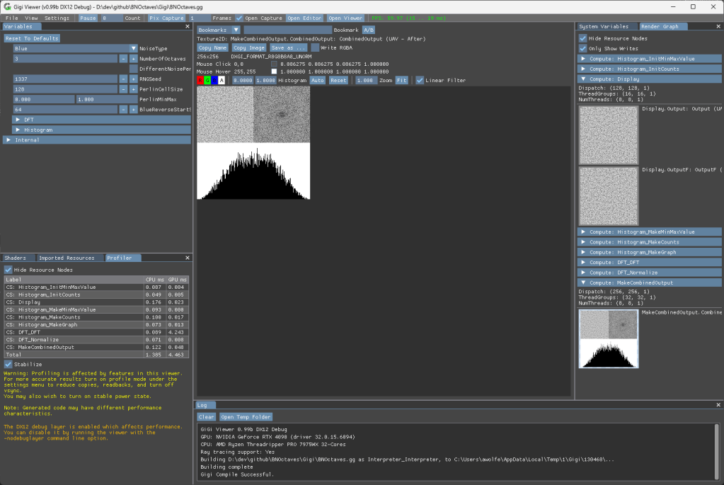
Use of Gigi – The Viewer

If you click “Open Viewer” in the main technique (BNOctaves.gg) it will open it in the viewer. You can change the settings in the upper left “Variables” tab and see the results instantly. You can also look at the graph at different points in the execution on the right in the “Render Graph” tab, and can inspect the values of pixels etc like you would with a render doc capture. A profiler also shows CPU and GPU time in the lower left. (I told you the DFT was slow, ha!). For each image above in this blog post, i set the parameters like I wanted and then clicked “copy image” to get it to paste into this blog post.

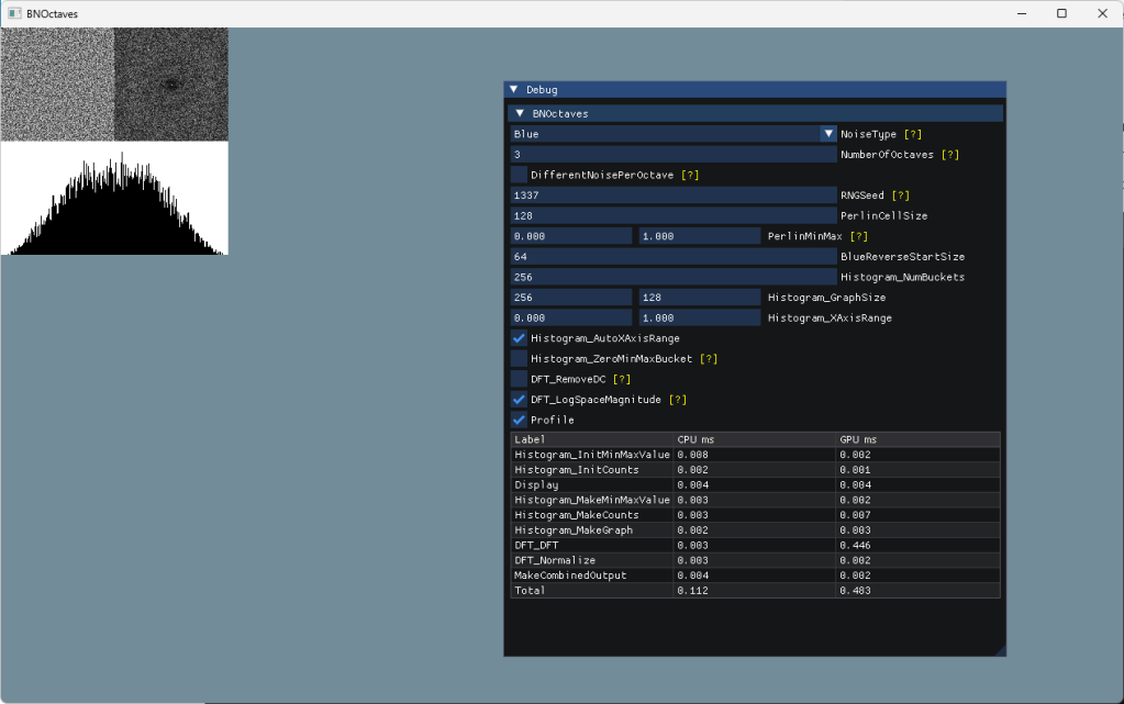
Use of Gigi – The Compiler & Generated Code

I used GigiCompiler.exe to generate “DX12_Application” code for this technique and the results of that are in the “dx12” folder in the repo. You run “MakeSolution.bat” to have cmake create BNOctaves.sln and then can open and run it. Running that, you have the same parameters as you do in the viewer, including a built in profiler.

I did have to make one modification after generating the C++ DX12 code. There are “TODO:”s in the main.cpp to help guide you, but in my case, all I needed to do was copy the “Combined Output” texture to the render target. That is on line 456:

            // TODO: Do post execution work here, such as copying an output texture to g_mainRenderTargetResource[backBufferIdx]
            CopyTextureToTexture(g_pd3dCommandList, m_BNOctaves->m_output.texture_CombinedOutput, m_BNOctaves->m_output.c_texture_CombinedOutput_endingState, g_mainRenderTargetResource[backBufferIdx], D3D12_RESOURCE_STATE_RENDER_TARGET);

Closing

I sincerely believe that “the age of noise” in graphics has just begun. I more mean noise meant for use in sampling or optimized for filtering, but that type of noise may have use in procedural content generation too, like this post explored.

I am also glad that Gigi is finally open sourced, and that I can use this absolute power tool of research in blog posts like this, while also helping other people understand the value it brings. Hopefully you caught a glimpse of that in this post.