The C++ code that implements this blog post and generated the images can be found at https://github.com/Atrix256/GoldenRatioShuffle2D.

I previously wrote about how to make a one dimensional low discrepancy shuffle iterator at https://blog.demofox.org/2024/05/19/a-low-discrepancy-shuffle-iterator-random-access-inversion/. That shuffle iterator also supported random access and inversion. That is a lot of words, so breaking it down:

• Shuffle Iterator – This means you have an iterator that can walk through the items in a shuffle without actually shuffling the list. It’s seedable too, to have different shuffles.
• Low Discrepancy – This means that if you are doing something like numerical integration on the items in the list, you’ll get faster convergence than using a white noise random shuffle.
• Random Access – You can ask for any item index in the shuffle and get the result in constant time. If you are shuffling 1,000,000 items and want to know what item will be at the 900,000th place, you don’t have to walk through 900,000 items to find out what’s there. It is just as happy telling you what is at the 900,000th place in the shuffle, as what is at the 0th place.
• Inversion – You can also ask the reverse question: At what point in the shuffle does item 1000 come up? It also gives this answer in constant time.

After writing that post, I spent some time trying to find a way to do the same thing in two dimensions. I tried some things with limited success, but didn’t find anything worth sharing.

A couple people suggested I try putting the 1D shuffle iterator output through the Hilbert curve, which is a way of mapping 1d points to 2d points. I finally got around to trying it recently, and yep, it works!

You can also use the Z-order curve (or Morton curve) to do the same thing, and it works, but it doesn’t give as nice results as the Hilbert curve does.

People also probably wonder how Martin Robert’s R2 sequence (from https://extremelearning.com.au/unreasonable-effectiveness-of-quasirandom-sequences/) would work here, since it generalizes the golden ratio to 2d, and the 1d shuffle iterator is based on the golden ratio, but I couldn’t find a way to make it work. For example, multiplying the R2 sequence by the width and height of the 2D grid and casting to integer causes the same 2d location to be chosen multiple times, which also leaves other 2d locations never chosen. That is fine for many applications, but if you want a shuffle, it really needs to visit each item exactly once during the shuffle. Below is how many duplicates that had at various resolutions. Random is also included (white noise, but not a shuffle) to compare to.

Texture Size	Pixel Count	R2 Duplicate Pixels	R2 Duplicate Percent	Random Duplicate Percent
64×64	4,096	847	20.68%	36.89%
128×128	16,384	3,379	20.62%	37.01%
256×256	65,536	16,375	24.99%	36.78%
512×512	262,144	29,203	11.14%	36.80%
1024×1024	1,048,576	392,921	37.47%	36.78%
2048×2048	4,194,304	1,831,114	43.66%	36.78%

So first up, here’s an RMSE (root mean squared error) graph, integrating an image in the repo cabin.png (aka finding the average pixel color). RMSE is averaged over 1000 tests to reduce noise in the plot, where each test used a different random seed for the shuffles. White uses a standard white noise shuffle. Hilbert and ZOrder use a 1D low discrepancy shuffle, then use their respective curves to turn it into a 2D point.

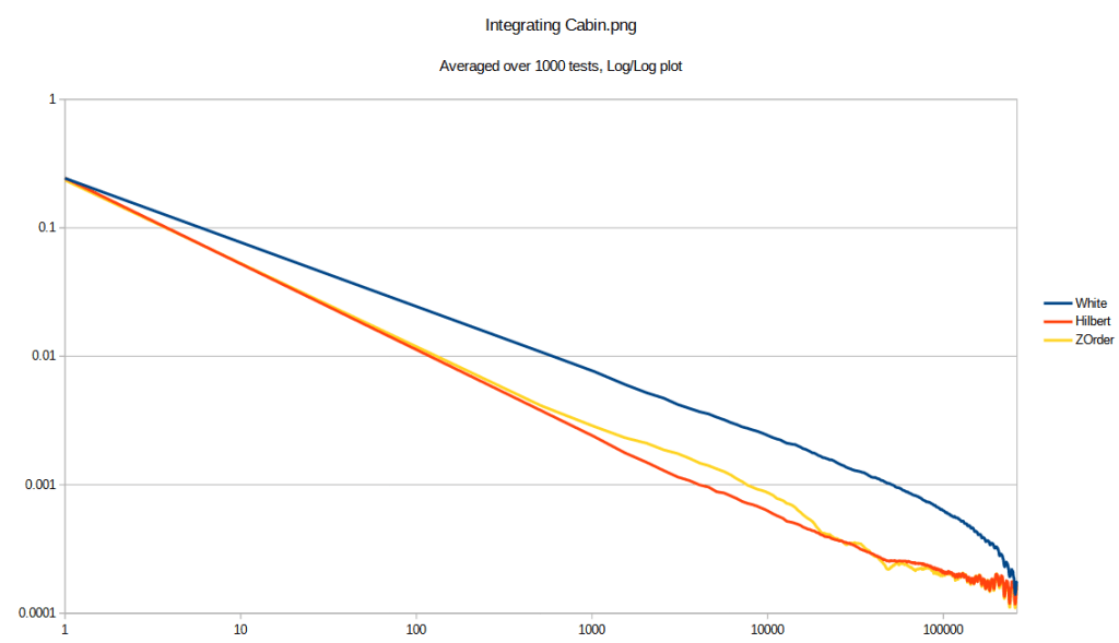
Here is the 512×512 image being integrated:

So that’s great… Hilbert gives best results generally, but Z Order also does well, compared to a white noise shuffle.

Some things worth noting:

• Both Hilbert and Z order curves can be reversed – they can map 1d to 2d, and then 2d back to 1d. That means that this 2d shuffle is reversible as well. To figure out at what point in a shuffle a specific 2D point will appear, you first do the inverse curve transformation to get the 1D index of that point, and then ask the low discrepancy shuffle when that 1D index will show up.
• As I’ve written it, this is limited to powers of 2. There are ways of making Hilbert curves that are not powers of 2 in size but I’ll leave that to you implement 😛

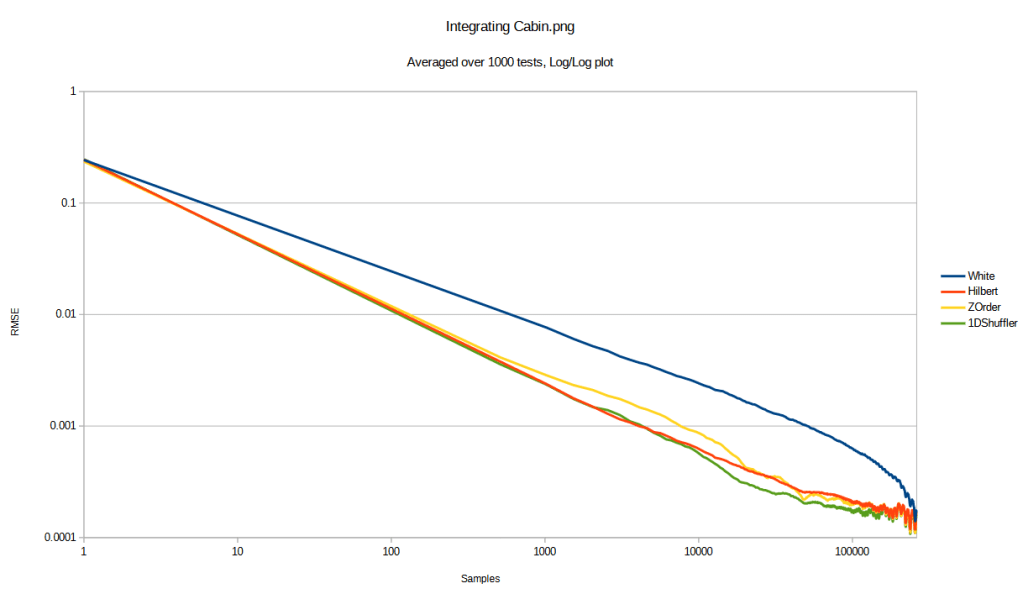
I did omit something from the previous test though… What if we didn’t put the 1d shuffle through any curve? What if we treated the image as one long line of pixels (like it is, in memory) and used a 1d shuffle on that? Well, it does pretty well!

However, you should see the actual point sets we are talking about before you make a final judgement.

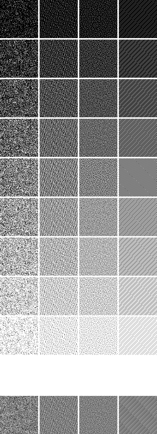
Below are the White noise shuffled points (left), Z order points (middle) left, Hilbert points (middle right) and 1DShuffler points (right) at different numbers of points, to show how they fill in the space. The last image in each uses a point’s order as a greyscale color to show how the values show up over time.

Click on the images to see them full sized.

64×64

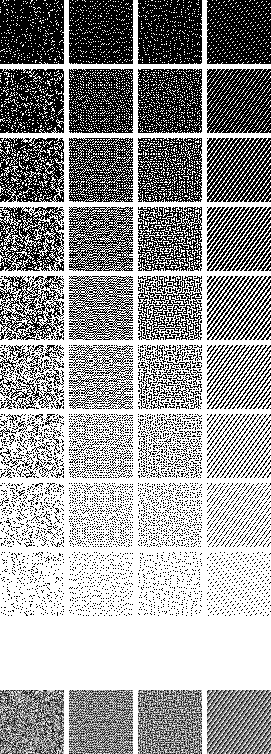
128×128

256×256

512×512

1024×1024

So, while the 1DShuffler may give better convergence, especially near the full sample count, the point set is very regularly ordered and would make noticeable rendering artifacts. This is very similar to the usual trade off of low discrepancy sequences converging faster but having aliasing problems, compared to blue noise which converges more slowly but does not suffer from aliasing, and is isotropic.

You might notice a strange thing in Hilbert at 1024×1024 where it seems to fill in “in clumps”. 2048×2048 seems to do the same, but 4096×4096 goes back to not clumping. It’s strange and my best guess as to what is going on is that Hilbert mapping 1d to 2d means that points nearby in 1d are also nearby in 2d, but the reverse does not hold. Points far away in 1d are not necessarily far away in 2d? I’m not certain though.

Bonus Convergence Tests

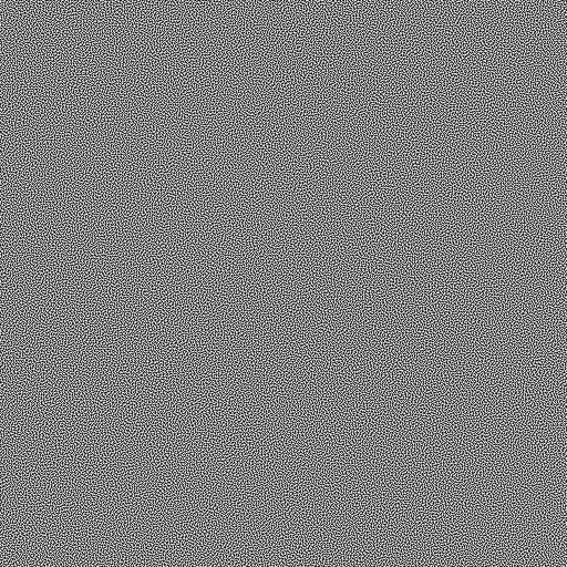
Here’s a 512×512 white noise image to integrate, and the convergence graph below.

Here is the same with a blue noise texture. This blue noise made with FAST (https://github.com/electronicarts/fastnoise). This is the same pixel values as the white noise texture above, just re-arranged into a blue noise pattern.

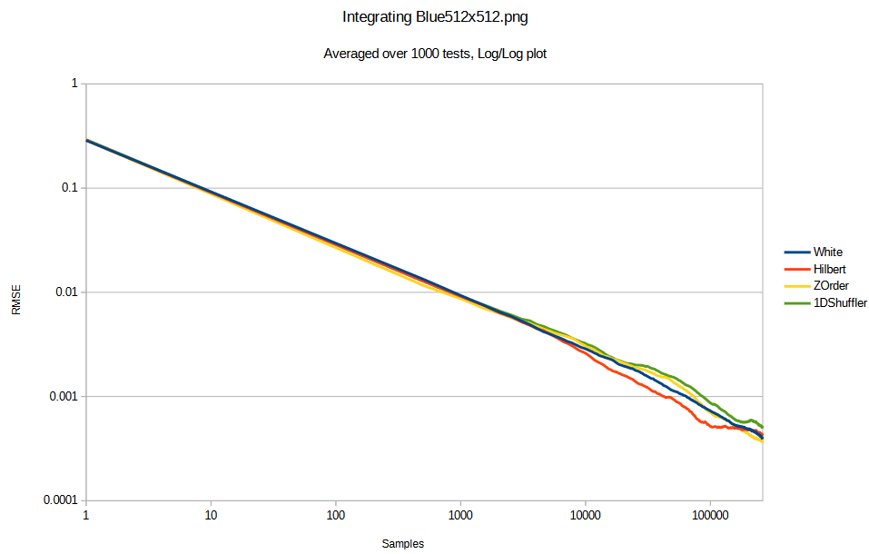
So interestingly, integrating the white noise texture made the “good samplers” do less good. Integrating the blue noise texture made the “good samplers” do even less well and be equal to white noise sampling.

What gives?

This isn’t proven, and isn’t anything that I’ve seen talked about in literature, but here’s my intuition of what’s going on:

“Good sampling” relies on small changes in sampling location giving small changes in sampled value. This way, when it samples a domain in a roughly evenly spaced way, it can be confident that it got fairly representative values of the whole image.

This is true of regular images, where moving a pixel to the left or right is going to usually give you the same color.

This may or may not be true in a white noise texture, randomly.

A blue noise texture however, is made to BREAK this assumption. Small changes in location on a blue noise texture will give big changes in value.

Just a weird observation – good sampling tends to be high frequency, while good integrands tend to be low frequency. Good sampling tends to have negative correlation, while good integrands tend to have positive correlation.