A few months ago I saw what I’m about to show you for the first time, and my jaw dropped. I’m hoping to share that experience with you right now, as a I share a quick intro to probabilistic algorithms, starting with KMV, otherwise known as K-Minimum Values, which is a Distinct Value (DV) Sketch, or a DV estimator.

Thanks to Ben Deane for exposure to this really interesting area of computer science.

The Setup

Let’s say that you needed a program to count the number of unique somethings that you’ve encountered. The unique somethings could be unique visitors on a web page, unique logins into a server within a given time period, unique credit card numbers, or anything else that has a way for you to get some unique identifier.

One way to do this would be to keep a list of all the things you’ve encountered before, only inserting a new item if it isn’t already in the list, and then count the items in the list when you want a count of unique items. The obvious downside here is that if the items are large and/or there are a lot of them, your list can get pretty large. In fact, it can take an unbounded amount of memory to store this list, which is no good.

A better solution may be instead of storing the entire item in the list, maybe instead you make a 32 bit hash of the item and then add that hash to a list if it isn’t already in the list, knowing that you have at most 2^32 (4,294,967,296) items in the list. It’s a bounded amount of memory, which is an improvement, but it’s still pretty large. The maximum memory requirement there is 2^32 * 4 which is 17,179,869,184 bytes or 16GB.

You may even do one step better and just decide to have 2^32 bits of storage, and when you encounter a specific 32 bit hash, use that as an index and set that specific bit to 1. You could then count the number of bits set and use that as your answer. That only takes 536,870,912 bytes, or 512MB. A pretty big improvement over 16GB but still pretty big. Also, try counting the number of bits set in a 512MB region of memory. That isn’t the fastest operation around 😛

We made some progress by moving to hashes, which put a maximum size amount of memory required, but that came at the cost of us introducing some error. Hashes can have collisions, and when that occurs in our scenarios above, we have no way of knowing that two items hashing to the same value are not the same item.

Sometimes it’s ok though that we only have an approximate answer, because getting an exact answer may require resources we just don’t have – like infinite memory to hold an infinitely large list, and then infinite computing time to count how many items there are. Also notice that the error rate is tuneable if we want to spend more memory. If we used a 64 bit hash instead of a 32 bit hash, our hash collisions would decrease, and our result would be more accurate, at the cost of more memory used.

The Basic Idea

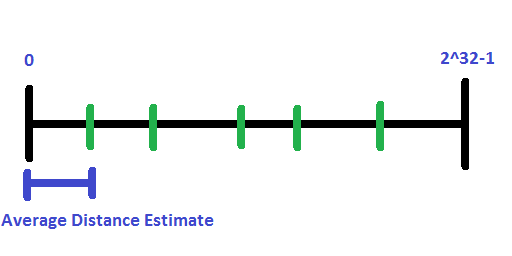
Let’s try something different, let’s hash every item we see, but only store the lowest valued hash we encounter. We can then use that smallest hash value to estimate how many unique items we saw. That’s not immediately intuitive, so here’s the how and the why…

When we put something into a hash function, what we are doing really is getting a deterministic pseudo random number to represent the item. If we put the same item in, we’ll get the same number out every time, and if we put in a different item, we should get a different number out, even if the second item is really similar to the first item. Interestingly the numbers we get out should have no bearing on the nature of the items we put into the hash. Even if the items we put in are similar, the output should be just as different (on average) as if we put in items that were completely different.

This is one of the properties of a good hash function, that it’s output is (usually) evenly distributed, no matter the nature of the input. What that means is that if we put N items into a hash function, those items are on average going to be evenly spaced in the output of the hash, regardless of how similar or different they were before going into the hash function.

Using this property, the distance from zero to the smallest hash we’ve ever seen can be treated as a representative estimate of the average distance between each item that we hashed. So, to get the number of items in the hash, we convert the smallest hash into a percentage from 0 to 1 of the total hash space (for uint32, convert to float and divide by (float)2^32), and then we can use this formula:

numItems = (1 / percentage) – 1

To understand why we subtract the 1, imagine that our minimum hash value is 0.5. If that is an accurate representation of the space between values, that means that we only have 1 value, right in the middle. But, if we didvide 1 by 0.5 we get 2. We have 2 REGIONS, but we have only 1 item in the list, so we need to subtract 1.

As another example imagine that our minimum hash is 0.3333 and that it is an accurate representation of the space between values. If we divide 1 by 0.3333, we get 3. We do have 3 regions if we cut the whole space into 3 parts, but we only have 2 items (we made 2 cuts to make 3 regions).

Reducing Error

This technique doesn’t suffer too much from hash collisions (so long as your hash function is a decent hash function), but it does have a different sort of problem.

As you might guess, sometimes the hash function might not play nice, and you could hash only a single item, get a hash of 1 and ruin the count estimation. So, there is possibility for error in this technique.

To help reduce error, you ultimately need information about more ranges so that you can combine the multiple pieces of information together to get a more accurate estimate.

Here are some ways to gather information about more ranges:

• Keep the lowest and highest hash seen instead of just the lowest. This doubles the range information you have since you’d know the range 0-min and max-1.
• Keep the lowest N hashes seen instead of only the lowest. This multiplies the amount of range information you have by N.
• Instead of keeping the lowest value from a single hash, perform N hashes instead and keep the lowest value seen from each hash. Again, this multiplies the amount of range information you have by N.
• Alternately, just salt the same hash N different ways (with high quality random numbers) instead of using N different hash functions, but still keep the lowest seen from each “value channel”. Multiplies info by N again.
• Also a possibility, instead of doing N hashes or N salts, do a single hash, and xor that hash against N different high quality random numbers to come up with N deterministic pseudorandom numbers per item. Once again, still keep the lowest hash value seen from each “value channel”. Multiplies info by N again
• Mix the above however you see fit!

Whatever route you go, the ultimate goal is to just get information about more ranges to be able to combine them together.

In vanilla KMV, the second option is used, which is to keep the N lowest hashes seen, instead of just a single lowest hash seen. Thus the full name for KMV: K-Minimum Values.

Combining Info From Multiple Ranges

When you have the info from multiple ranges and need to combine that info, it turns out that using the harmonic mean is the way to go because it’s great at filtering out large values in data that don’t fit with the rest of the data.

Since we are using division to turn the hash value into an estimate (1/percentValue-1), unusually small hashes will result in exponentially larger values, while unusually large hashes will not affect the math as much, but also likely will be thrown out before we ever see them since they will likely not be the minimum hash that we’ve seen.

I don’t have supporting info handy, but from what I’ve been told, the harmonic mean is provably better than both the geometric mean and the regular plain old vanilla average (arithmetic mean) in this situation.

So, to combine information from the multiple ranges you’ve gathered, you turn each range into a distinct value estimate (by calculating 1/percentValue-1) and then putting all those values through the mean equation of your choice (which ought to be harmonic mean, but doesn’t strictly have to be!). The result will be your final answer.

Set Operations

Even though KMV is just a distinct value estimator that estimates a count, there are some interesting probabilistic set operations that you can do with it as well. I’ll be talking about using the k min value technique for gathering information from multiple ranges, but if you use some logic you should be able to figure out how to make it work when you use any of the other techniques.

Jaccard Index

Talking about set operations, I want to start with a concept called the Jaccard index (sometimes called the Jaccard similarity coefficient).

If you have 2 sets, the Jaccard index is calculated by:

Jaccard Index = count(intersection(A,B)) / count(union(A,B))

Since the union of A and B is the combined list of all items in those sets, and the intersection of A and B is the items that they have in common, you can see that if the sets have all items in common, the Jaccard index will be 1 and if the sets have no items in common, the Jaccard index will be 0. If you have some items in common it will be somewhere between 0 and 1. So, the Jaccard Index is just a measurement of how similar two sets are.

Union

If you have the information for two KMV objects, you can get an estimate to the number of unique items there if you were to union them together, even though you don’t have much of the info about the items that are in the set.

To do a union, you just combine the minimum value lists, and remove the K largest ones, so that you are left with the K minimum values from both sets.

You then do business as usual to estimate how many items are in that resulting set.

If you think about it, this makes sense, because if you tracked the items from both lists in a third KMV object, you’d end up with the same K minimums as if you took the K smallest values from both sets individually.

Note that if the two KMV objects are of different size, due to K being different sizes, or because either one isn’t completely filled with K minimum values, you should use the smaller value of K as your union set K size.

Intersection

Finding an estimated count of intersections between two sets is a little bit different.

Basically, having the K minimum hashes seen from both lists, you can think of that as a kind of random sample of a range in both lists. You can then calculate the Jaccard index for that range you have for the two sets (by dividing the size of the intersection by the size of the union), and then use that Jaccard index to estimate an intersection count for the entire set based on the union count estimate.

You can do some algebra to the Jaccard index formula above to get this:

count(intersection(A,B)) = Jaccard Index * count(union(A,B))

Just like with union, if the two KMV objects are of different size, due to K being different sizes, or because either one isn’t completely filled with K minimum values, you should use the smaller value of K.

Sample Code

#include 
#include 
#include 
#include 
#include 
#include 

// The CKMVCounter class
template <typename T, unsigned int NUMHASHES, typename HASHER = std::hash>
class CKMVUniqueCounter
{
public:
	// constants
	static const unsigned int c_numHashes = NUMHASHES;
	static const size_t c_invalidHash = (size_t)-1;

	// constructor
	CKMVUniqueCounter ()
	{
		// fill our minimum hash values with the maximum possible value
		m_minHashes.fill(c_invalidHash);
		m_largestHashIndex = 0;
	}

	// interface
	void AddItem (const T& item)
	{
		// if the new hash isn't smaller than our current largest hash, do nothing
		const size_t newHash = HASHER()(item);
		if (m_minHashes[m_largestHashIndex] <= newHash)
			return;

		// if the new hash is already in the list, don't add it again
		for (unsigned int index = 0; index < c_numHashes; ++index)
		{
			if (m_minHashes[index] == newHash)
				return;
		}

		// otherwise, replace the largest hash
		m_minHashes[m_largestHashIndex] = newHash;

		// and find the new largest hash
		m_largestHashIndex = 0;
		for (unsigned int index = 1; index  m_minHashes[m_largestHashIndex])
				m_largestHashIndex = index;
		}
	}

	// probabilistic interface
	void UniqueCountEstimates (float &arithmeticMeanCount, float &geometricMeanCount, float &harmonicMeanCount)
	{
		// calculate the means of the count estimates.  Note that if there we didn't get enough items
		// to fill our m_minHashes array, we are just ignoring the unfilled entries.  In production
		// code, you would probably just want to return the number of items that were filled since that
		// is likely to be a much better estimate.
		// Also, we need to sort the hashes before calculating uniques so that we can get the ranges by
		// using [i]-[i-1] instead of having to search for the next largest item to subtract out
		SortHashes();
		arithmeticMeanCount = 0.0f;
		geometricMeanCount = 1.0f;
		harmonicMeanCount = 0.0f;
		int numHashes = 0;
		for (unsigned int index = 0; index < c_numHashes; ++index)
		{
			if (m_minHashes[index] == c_invalidHash)
				continue;
			numHashes++;
			float countEstimate = CountEstimate(index);
			arithmeticMeanCount += countEstimate;
			geometricMeanCount *= countEstimate;
			harmonicMeanCount += 1.0f / countEstimate;
		}
		arithmeticMeanCount = arithmeticMeanCount / (float)numHashes;
		geometricMeanCount = pow(geometricMeanCount, 1.0f / (float)numHashes);
		harmonicMeanCount /= (float)numHashes;
		harmonicMeanCount = 1.0f / harmonicMeanCount;
	}

	// friends
	template 
	friend CKMVUniqueCounter KMVUnion (
		const CKMVUniqueCounter& a,
		const CKMVUniqueCounter& b
	);

	template 
	friend float KMVJaccardIndex (
		const CKMVUniqueCounter& a,
		const CKMVUniqueCounter& b
	);

private:

	unsigned int NumHashesSet () const
	{
		unsigned int ret = 0;
		for (unsigned int index = 0; index  0 ? m_minHashes[hashIndex- 1] : 0;
		const float percent = (float)(currentHash-lastHash) / (float)((size_t)-1);
		return (1.0f / percent) - 1.0f;
	}
	
	// the minimum hash values
	std::array m_minHashes;
	size_t m_largestHashIndex;
};

// Set interface
template 
CKMVUniqueCounter KMVUnion (
	const CKMVUniqueCounter& a,
	const CKMVUniqueCounter& b
)
{
	// gather the K smallest hashes seen, where K is the smaller, removing duplicates
	std::set setMinHashes;
	std::for_each(a.m_minHashes.begin(), a.m_minHashes.end(), [&setMinHashes](size_t v) {setMinHashes.insert(v); });
	std::for_each(b.m_minHashes.begin(), b.m_minHashes.end(), [&setMinHashes](size_t v) {setMinHashes.insert(v); });
	std::vector minHashes(setMinHashes.begin(), setMinHashes.end());
	std::sort(minHashes.begin(),minHashes.end());
	minHashes.resize(std::min(a.NumHashesSet(), b.NumHashesSet()));

	// create and return the new KMV union object
	CKMVUniqueCounter ret;
	for (unsigned int index = 0; index < minHashes.size(); ++index)
		ret.m_minHashes[index] = minHashes[index];
	ret.m_largestHashIndex = ret.c_numHashes - 1;
	return ret;
}

template 
float KMVJaccardIndex (
	const CKMVUniqueCounter& a,
	const CKMVUniqueCounter& b
)
{
	size_t smallerK = std::min(a.NumHashesSet(), b.NumHashesSet());

	size_t matches = 0;
	for (size_t ia = 0; ia < smallerK; ++ia)
	{
		for (size_t ib = 0; ib < smallerK; ++ib)
		{
			if (a.m_minHashes[ia] == b.m_minHashes[ib])
			{
				matches++;
				break;
			}
		}
	}

	return (float)matches / (float)smallerK;
}

// data to add to the lists
const char *s_boyNames[] =
{
	"Loki",
	"Alan",
	"Paul",
	"Stripes",
	"Shelby",
	"Ike",
	"Rafael",
	"Sonny",
	"Luciano",
	"Jason",
	"Brent",
	"Jed",
	"Lesley",
	"Randolph",
	"Isreal",
	"Charley",
	"Valentin",
	"Dewayne",
	"Trent",
	"Abdul",
	"Craig",
	"Andre",
	"Brady",
	"Markus",
	"Randolph",
	"Isreal",
	"Charley",
	"Brenton",
	"Herbert",
	"Rafael",
	"Sonny",
	"Luciano",
	"Joshua",
	"Ramiro",
	"Osvaldo",
	"Monty",
	"Mckinley",
	"Colin",
	"Hyman",
	"Scottie",
	"Tommy",
	"Modesto",
	"Reginald",
	"Lindsay",
	"Alec",
	"Marco",
	"Dee",
	"Randy",
	"Arthur",
	"Hosea",
	"Laverne",
	"Bobbie",
	"Damon",
	"Les",
	"Cleo",
	"Robt",
	"Rick",
	"Alonso",
	"Teodoro",
	"Rodolfo",
	"Ryann",
	"Miki",
	"Astrid",
	"Monty",
	"Mckinley",
	"Colin",
	nullptr
};

const char *s_girlNames[] =
{
	"Chanel",
	"Colleen",
	"Scorch",
	"Grub",
	"Anh",
	"Kenya",
	"Georgeann",
	"Anne",
	"Inge",
	"Georgeann",
	"Anne",
	"Inge",
	"Analisa",
	"Ligia",
	"Chasidy",
	"Marylee",
	"Lashandra",
	"Frida",
	"Katie",
	"Alene",
	"Brunilda",
	"Zoe",
	"Shavon",
	"Anjanette",
	"Daine",
	"Sheron",
	"Hilary",
	"Felicitas",
	"Cristin",
	"Ressie",
	"Tynisha",
	"Annie",
	"Sharilyn",
	"Astrid",
	"Charise",
	"Gregoria",
	"Angelic",
	"Lesley",
	"Mckinley",
	"Lindsay",
	"Shanelle",
	"Karyl",
	"Trudi",
	"Shaniqua",
	"Trinh",
	"Ardell",
	"Doreen",
	"Leanna",
	"Chrystal",
	"Treasa",
	"Dorris",
	"Rosalind",
	"Lenore",
	"Mari",
	"Kasie",
	"Ann",
	"Ryann",
	"Miki",
	"Lasonya",
	"Olimpia",
	"Shelby",
	"Lesley",
	"Mckinley",
	"Lindsay",
	"Dee",
	"Bobbie",
	"Cleo",
	"Leanna",
	"Chrystal",
	"Treasa",
	nullptr
};

// driver program
void WaitForEnter ()
{
	printf("nPress Enter to quit");
	fflush(stdin);
	getchar();
}

void main(void)
{
	// how many min values all these KMV objects keep around
	static const int c_numMinValues = 15;

	printf("Using %u minimum valuesnn", c_numMinValues);

	// =====================  Boy Names  =====================
	// put our data into the KVM counter
	CKMVUniqueCounter boyCounter;
	unsigned int index = 0;
	while (s_boyNames[index] != nullptr)
	{
		boyCounter.AddItem(s_boyNames[index]);
		index++;
	}

	// get our count estimates
	float arithmeticMeanCount, geometricMeanCount, harmonicMeanCount;
	boyCounter.UniqueCountEstimates(arithmeticMeanCount, geometricMeanCount, harmonicMeanCount);

	// get our actual unique count
	std::set actualBoyUniques;
	index = 0;
	while (s_boyNames[index] != nullptr)
	{
		actualBoyUniques.insert(s_boyNames[index]);
		index++;
	}

	// print the results!
	printf("Boy Names:n%u actual uniquesn", actualBoyUniques.size());
	float actualCount = (float)actualBoyUniques.size();
	printf("Estimated counts and percent error:n  Arithmetic Mean: %0.2ft%0.2f%%n"
		"  Geometric Mean : %0.2ft%0.2f%%n  Harmonic Mean  : %0.2ft%0.2f%%n",
		arithmeticMeanCount, 100.0f * (arithmeticMeanCount - actualCount) / actualCount,
		geometricMeanCount, 100.0f * (geometricMeanCount - actualCount) / actualCount,
		harmonicMeanCount, 100.0f * (harmonicMeanCount - actualCount) / actualCount);

	// =====================  Girl Names  =====================
	// put our data into the KVM counter
	CKMVUniqueCounter girlCounter;
	index = 0;
	while (s_girlNames[index] != nullptr)
	{
		girlCounter.AddItem(s_girlNames[index]);
		index++;
	}

	// get our count estimates
	girlCounter.UniqueCountEstimates(arithmeticMeanCount, geometricMeanCount, harmonicMeanCount);

	// get our actual unique count
	std::set actualGirlUniques;
	index = 0;
	while (s_girlNames[index] != nullptr)
	{
		actualGirlUniques.insert(s_girlNames[index]);
		index++;
	}

	// print the results!
	printf("nGirl Names:n%u actual uniquesn", actualGirlUniques.size());
	actualCount = (float)actualGirlUniques.size();
	printf("Estimated counts and percent error:n  Arithmetic Mean: %0.2ft%0.2f%%n"
		"  Geometric Mean : %0.2ft%0.2f%%n  Harmonic Mean  : %0.2ft%0.2f%%n",
		arithmeticMeanCount, 100.0f * (arithmeticMeanCount - actualCount) / actualCount,
		geometricMeanCount, 100.0f * (geometricMeanCount - actualCount) / actualCount,
		harmonicMeanCount, 100.0f * (harmonicMeanCount - actualCount) / actualCount);

	// =====================  Set Operations  =====================

	// make the KMV union and get our count estimates
	CKMVUniqueCounter boyGirlUnion = KMVUnion(boyCounter, girlCounter);
	boyGirlUnion.UniqueCountEstimates(arithmeticMeanCount, geometricMeanCount, harmonicMeanCount);

	// make the actual union
	std::set actualBoyGirlUnion;
	std::for_each(actualBoyUniques.begin(), actualBoyUniques.end(),
		[&actualBoyGirlUnion](const std::string& s)
		{
			actualBoyGirlUnion.insert(s);
		}
	);
	std::for_each(actualGirlUniques.begin(), actualGirlUniques.end(),
		[&actualBoyGirlUnion](const std::string& s)
		{
			actualBoyGirlUnion.insert(s);
		}
	);

	// print the results!
	printf("nUnion:n%u actual uniques in unionn", actualBoyGirlUnion.size());
	actualCount = (float)actualBoyGirlUnion.size();
	printf("Estimated counts and percent error:n  Arithmetic Mean: %0.2ft%0.2f%%n"
		"  Geometric Mean : %0.2ft%0.2f%%n  Harmonic Mean  : %0.2ft%0.2f%%n",
		arithmeticMeanCount, 100.0f * (arithmeticMeanCount - actualCount) / actualCount,
		geometricMeanCount, 100.0f * (geometricMeanCount - actualCount) / actualCount,
		harmonicMeanCount, 100.0f * (harmonicMeanCount - actualCount) / actualCount);

	// calculate estimated jaccard index
	float estimatedJaccardIndex = KMVJaccardIndex(boyCounter, girlCounter);

	// calculate actual jaccard index and actual intersection
	size_t actualIntersection = 0;
	std::for_each(actualBoyUniques.begin(), actualBoyUniques.end(),
		[&actualGirlUniques, &actualIntersection] (const std::string &s)
		{
			if (actualGirlUniques.find(s) != actualGirlUniques.end())
				actualIntersection++;
		}
	);
	float actualJaccardIndex = (float)actualIntersection / (float)actualBoyGirlUnion.size();

	// calculate estimated intersection
	float estimatedIntersection = estimatedJaccardIndex * (float)actualBoyGirlUnion.size();

	// print the intersection and jaccard index information
	printf("nIntersection:n%0.2f estimated, %u actual.  Error: %0.2f%%n",
		estimatedIntersection,
		actualIntersection,
		100.0f * (estimatedIntersection - (float)actualIntersection) / (float)actualIntersection);

	printf("nJaccard Index:n%0.2f estimated, %0.2f actual.  Error: %0.2f%%n",
		estimatedJaccardIndex,
		actualJaccardIndex,
		100.0f * (estimatedJaccardIndex-actualJaccardIndex) / actualJaccardIndex
	);

	WaitForEnter();
}

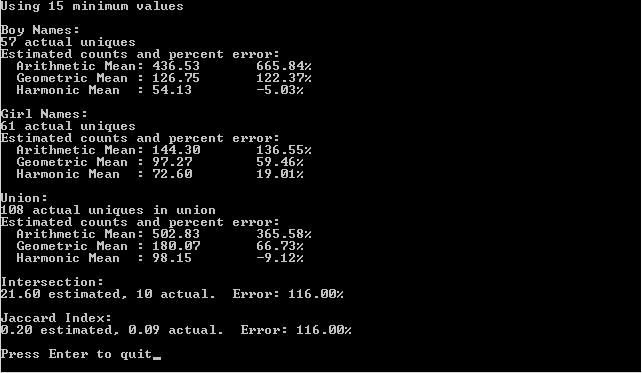
Here’s the output of the program:

Upgrading from Set to Multi Set

Interestingly, if you keep a count of how many times you’ve seen each hash in the k min hash, you can upgrade this algorithm from being a set algorithm to a multi set algorithm and get some other interesting information from it.

Where a set is basically a list of unique items, a multi set is a set of unique items that also have a count associated with them. In this way, you can think of a multiset as just a list of items which may appear more than once.

Upgrading KMV to a multi set algorithm lets you do some new and interesting things where instead of getting information only about unique counts, you can get information about non unique counts too. But to re-iterate, you still keep the ability to get unique information as well, so it is kind of like an upgrade, if you are interested in multiset information.

Links

Want more info about this technique?

Sketch of the Day: K-Minimum Values

Sketch of the Day: Interactive KMV web demo

K-Minimum Values: Sketching Error, Hash Functions, and You

Wikipedia: MinHash – Jaccard similarity and minimum hash values

All Done

I wanted to mention that even though this algorithm is a great, intuitive introduction into probabilistic algorithms, there are actually much better distinct value estimators in use today, such as one called HyperLogLog which seems to be the current winner. Look for a post on HyperLogLog soon 😛

KMV is better than other algorithms at a few things though. Specifically, from what I’ve read, that it can extend to multiset makes it very useful, and also it is much easier to calculate intersections versus other algorithms.

I also wanted to mention that there are interesting usage cases for this type of algorithms in game development, but where these probabilistic algorithms really shine is in massive data situations like google, amazon, netflix etc. If you go out searching for more info on this stuff, you’ll probably be led down many big data / web dev rabbit holes, because that’s where the best information about this stuff resides.

Lastly, I wanted to mention that I’m using the C++ std::hash built in hash function. I haven’t done a lot of research to see how it compares to other hashes, but I’m sure, much like rand(), the built in functionality leaves much to be desired for “power user” situations. In other words, if you are going to use this in a realistic situation, you probably are better off using a better hashing algorithm. If you need a fast one, you might look into the latest murmurhash variant!

More probabilistic algorithm posts coming soon, so keep an eye out!