

In the 90s before I was a professional programmer / game developer I looked at neural networks and found them interesting but got scared off by things like back propagation, which I wasn’t yet ready to understand.
With all the interesting machine learning things going on in modern times, I decided to have a look again and have been pleasantly surprised at how simple they are to understand. If you have knowledge of partial derivatives and gradients (like, if you’ve done any ray marching), you have the knowledge it takes to understand it.
Here are some really great resources I recomend for learning the nuts and bolts of how modern neural networks actually work:
Learn TensorFlow and deep learning, without a Ph.D.
Neural Networks and Deep Learning
A Neural Network Playground (Web Based NN sand box from google)
This post doesn’t require any understanding of neural networks or partial derivatives, so don’t worry if you don’t have that knowledge. The harder math comes up when training a neural network, but we are only going to be dealing with evaluating neural networks, which is much simpler.
A Geometric Interpretation of a Neuron
A neural network is made up layers.
Each layer has some number of neurons in it.
Every neuron is connected to every neuron in the previous and next layer.
Below is a diagram of a neural network, courtesy of wikipedia. Every circle is a neuron.

To calculate the output value of a neuron, you multiply every input into that neuron by a weight for that input, and add a bias. This value is fed into an activation function (more on activation functions shortly) and the result is the output value of that neuron. Here is a diagram for a single neuron:

A more formal definition of a neuron’s output is below. 


You might notice that the above is really just the dot product of the weight vector and the input vector, with a value added on the end. We could re-write it like that:

Interestingly, that is the same equation that you use to find the distance of a point to a plane. Let’s say that we have a plane defined by a unit length normal N and a distance to the origin d, and we want to calculate the distance of a point P to that plane. We’d use this formula:

This would give us a signed distance, where the value will be negative if we are in the negative half space defined by the plane, and positive otherwise.
This equation works if you are working in 3 dimensional space, but also works in general for any N dimensional point and plane definition.
What does this mean? Well, this tells us that every neuron in a neural network is essentially deciding what side of a hyperplane a point is on. Each neuron is doing a linear classification, saying if something is on side A or side B, and giving a distance of how far it is into A or B.
This also means that when you combine multiple neurons into a network, that an output neuron of that neural network tells you whether the input point is inside or outside of some shape, and by how much.
I find this interesting for two reason.
Firstly, it means that a neural network can be interpreted as encoding SHAPES, which means it could be used for modeling shapes. I’m interested in seeing what sort of shapes it’s capable of, and any sorts of behaviors this representation might have. I don’t expect it to be useful for, say, main stream game development (bonus if it is useful!) but at minimum it ought to be an interesting investigation to help understand neural networks a bit better.
Secondly, there is another machine learning algorithm called Support Vector Machines which are also based on being able to tell you which side of a separation a data point is on. However, unlike the above, SVM separations are not limited to plane tests and can use arbitrary shapes for separation. Does this mean that we are leaving something on the table for neural networks? Could we do better than we are to make networks with fewer layers and fewer neurons that do better classification by doing non linear separation tests?
Quick side note: besides classification, neural nets can help us with something called regression, which is where you fit a network to some analog data, instead of the more discrete problem of classification, which tells you what group something belongs to.
It turns out that the activation function of a neuron can have a pretty big influence on what sort of shapes are possible, which makes it so we aren’t strictly limited to shapes made up of planes and lines, and also means we aren’t necessarily leaving things on the table compared to SVM’s.
This all sort of gives me the feeling though that modern neural networks may not be the best possible algorithm for the types of things we use them for. I feel like we may need to generalize them beyond biological limitations to allow things like multiplications between weighted inputs instead of only sums. I feel like that sort of setup will be closer to whatever the real ideal “neural computation” model might be. However, the modern main stream neural models do have the benefit that they are evaluated very efficiently via dot products. They are particularly well suited for execution on GPUs which excel at performing homogenous operations on lots and lots of data. So, a more powerful and more general “neuron” may come at the cost of increased computational costs, which may make them less desirable in the end.
As a quick tangent, here is a paper from 2011 which shows a neural network model which does in fact allow for multiplication between neuron inputs. You then will likely be wanting exponents and other things, so while it’s a step in the right direction perhaps, it doesn’t yet seem to be the end all be all!
Sum-Product Networks: A New Deep Architecture
It’s also worth while to note that there are other flavors of neural networks, such as convolutional neural networks, which work quite a bit differently.
Let’s investigate this geometric interpretation of neurons as binary classifiers a bit, focusing on some different activation functions!
Step Activation Function
The Heaviside step function is very simple. If you give it a value greater than zero, it returns a 1, else it returns a 0. That makes our neuron just spit out binary: either a 0 or a 1. The output of a neuron using the step activation function is just the below:

The output of a neuron using the step activation function is true if the input point is in the positive half space of the plane that this neuron describes, else it returns false.
Let’s think about this in 2d. Let’s make a neural network that takes x and y as input and spits out a value. We can make an image that visualizes the range from (-1,-1) to (1,1). Negative values can be shown in blue, zero in white, and positive values in orange.
To start out, we’ll make a 2d plane (aka a line) that runs vertically and passes through the origin. That means it is a 2d plane with a normal of (1,0) and a distance from the origin of 0. In other words, our network will have a single neuron that has weights of (1,0) and a bias of 0. This is what the visualization looks like:

You can actually play around with the experiments of this post and do your own using an interactive visualization I made for this post. Click here to see this first experiment: Experiment: Vertical Seperation
We can change the normal (weights) to change the angle of the line, and we can also change the bias to move the line to it’s relative left or right. Here is the same network that has it’s weights adjusted to (1,1) with a bias of 0.1.

Experiment: Diagonal Separation
The normal (1,1) isn’t normalized though, which makes it so the distance from origin (aka the bias) isn’t really 0.1 units. The distance from origin is actually divided by the length of the normal to get the REAL distance to origin, so in the above image, where the normal is a bit more than 1.0, the line is actually less than 0.1 units from the origin.
Below is the visualization if we normalize the weights to (0.707,0.707) but leave the bias at 0.1 units. The result is that the line is actually 0.1 units away from the origin.

Experiment: Normalized Diagonal Separation
Recalling the description of our visualization, white is where the network outputs zero, while orange is where the network outputs a positive number (which is 1 in this case).
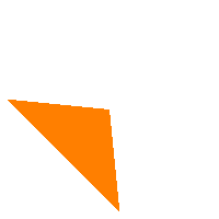
If we define three lines such that their negative half spaces don’t completely overlap, we can get a triangle where the network outputs a zero, while everywhere else it outputs a positive value. We do this by having three sibling neurons in the first layer which define three separate lines, and then in the output neuron we give them all a weight of 1. This makes it so the area outside the triangle is always a positive value, which step turns into 1, but inside the triangle, the value remains at 0.

Experiment: Negative Space Triangle
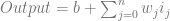
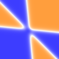
We can turn this negative space triangle into a positive space triangle however by making the output neuron have a weight on the inputs of -1, and adding a bias of 0.1. This makes it so that pixels in the positive space of any of the lines will become a negative value. The negative space of those three lines get a small bias to make it be a positive value, resulting in the step function making the values be 0 outside of the triangle, and 1 inside the triangle. This gives us a positive space triangle:
Experiment: Positive Space Triangle
Taking this a bit further, we can make the first layer define 6 lines, which make up two different triangles – a bigger one and a smaller one. We can then have a second layer which has two neurons – one which makes a positive space larger triangle, and one which makes a positive space smaller triangle. Then, in the output neuron we can give the larger triangle neuron a weight of 1, while giving the smaller triangle neuron a weight of -1. The end result is that we have subtracted the smaller triangle from the larger one:
Using the step function we have so far been limited to line based shapes. This has been due to the fact that we can only test our inputs against lines. There is a way around this though: Pass non linear input into the network!
Below is a circle with radius 0.5. The neural network has only a single input which is sqrt(x*x+y*y). The output neuron has a bias of -0.5 and a weight of 1. It’s the bias value which controls the radius of the circle.
You could pass other non linear inputs into the network to get a whole host of other shapes. You could pass sin(x) as an input for example, or x squared.

While the step function is inherently very much limited to linear tests, you can still do quite a lot of interesting non linear shapes (and data separations) by passing non linear input into the network.
Unfortunately though, you as a human would have to know the right non linear inputs to provide. The network can’t learn how to make optimal non linear separations when using the step function. That’s quite a limitation, but as I understand it, that’s how it works with support vector machines as well: a human can define non linear separations, but the human must decide the details of that separation.
BTW it seems like there could be a fun puzzle game here. Something like you have a fixed number of neurons that you can arrange in however many layers you want, and your goal is to separate blue data points from orange ones, or something like that. If you think that’d be a fun game, go make it with my blessing! I don’t have time to pursue it, so have at it (:
Identity and Relu Activation Functions
The identity activation function doesn’t do anything. It’s the same as if no activation function is used. I’ve heard that it can be useful in regression, but it can also be useful for our geometric interpretation.
Below is the same circle experiment as before, but using the identity activation function instead of the step activation function:

Remembering that orange is positive, blue is negative, and white is zero, you can see that outside the circle is orange (positive) and inside the circle is blue (negative), while the outline of the circle itself is white. We are looking at a signed distance field of the circle! Every point on this image is a scalar value that says how far inside or outside that point is from the surface of the shape.
Signed distance fields are a popular way of rendering vector graphics on the GPU. They are often approximated by storing the distance field in a texture and sampling that texture at runtime. Storing them in a texture only requires a single color channel for storage, and as you zoom in to the shape, they preserve their shape a lot better than regular images. You can read more about SDF textures on my post: Distance Field Textures.
Considering the machine learning perspective, having a signed distance field is also an interesting proposition. It would allow you to do classification of input, but also let you know how deeply that input point is classified within it’s group. This could be a confidence level maybe, or could be interpreted in some other way, but it gives a sort of analog value to classification, which definitely seems like it could come in handy sometimes.
If we take our negative space triangle example from the last section and change it from using step activation to identity activation, we find that our technique doesn’t generalize naively though, as we see below. (It doesn’t generalize for the positive space triangle either)

Experiment: Negative Space Triangle Identity
The reason it doesn’t generalize is that the negatives and positives of pixel distances to each of the lines cancel out. Consider a pixel on the edge of the triangle: you are going to have a near zero value for the edge it’s on, and two larger magnitude negative values from the other edges it is in the negative half spaces of. Adding those all together is going to be a negative value.
To help sort this out we can use an activation function called “relu”, which returns 0 if the value it’s given is less than zero, otherwise it returns the value. This means that all our negative values become 0 and don’t affect the distance summation. If we switch all the neurons to using relu activation, we get this:

Experiment: Negative Space Triangle Relu
If you squint a bit, you can see a triangle in the white. If you open the experiment and turn on “discrete output” to force 0 to blue you get a nice image that shows you that the triangle is in fact still there.

Our result with relu is better than identity, but there are two problems with our resulting distance field.
Firstly it isn’t a signed distance field – there is no blue as you might notice. It only gives positive distances, for pixels that are outside the shape. This isn’t actually that big of an issue from a rendering perspective, as unsigned distance fields are still useful. It also doesn’t seem that big of an issue from a machine learning perspective, as it still gives some information about how deeply something is classified, even though it is only from one direction.
I think with some clever operations, you could probably create the internal negative signed distance using different operations, and then could compose it with the external positive distance in the output neuron by adding them together.
The second problem is a bigger deal though: The distance field is no longer accurate!
By summing the distance values, the distance is incorrect for points where the closest feature of the triangle is a vertex, because multiple lines are contributing their distance to the final value.
I can’t think of any good ways to correct that problem in the context of a neural network, but the distance is an approximation, and is correct for the edges, and also gets more correct the closer you get to the object, so this is still useful for rendering, and probably still useful for machine learning despite it being an imperfect measurement.
Sigmoid and Hyperbolic Tangent Activation Function
The sigmoid function is basically a softer version of the step function and gives output between 0 and 1. The hyperbolic tangent activation function is also a softer version of the step function but gives output between -1 and 1.
Sigmoid:
Hyperbolic Tangent:
(images from Wolfram Mathworld)
They have different uses in machine learning, but I’ve found them to be visibly indistinguishable in my experiments after compensating for the different range of output values. It makes me think that smoothstep could probably be a decent activation function too, so long as your input was in the 0 to 1 range (maybe you could clamp input to 0 and 1?).
These activation functions let you get some non linearity in your neural network in a way that the learning algorithms can adjust, which is pretty neat. That puts us more into the realm where a neural net can find a good non linear separation for learned data. For the geometric perspective, this also lets us make more interesting non linear shapes.
Unfortunately, I haven’t been able to get a good understanding of how to use these functions to craft desired results.
It seems like if you add even numbers of hyperbolic tangents together in a neural network that you end up getting a lot of white, like below:

However, if you add an odd number of them together, it starts to look a bit more interesting, like this:
Other than that, it’s been difficult seeing a pattern that I can use to craft things. The two examples above were made by modifying the negative space triangle to use tanh instead of step.
Closing
We’ve wandered a bit in the idea of interpreting neural networks geometrically but I feel like we’ve only barely scratched the surface. This also hasn’t been a very rigorous exploration, but more has just been about exploring the problem space to get a feeling for what might be possible.
It would be interesting to look more deeply into some of these areas, particularly for the case of distance field generation of shapes, or combining activation functions to get more diverse results.
While stumbling around, it seems like we may have gained some intuition about how neural networks work as well.
It feels like whenever you add a layer, you are adding the ability for a “logical operation” to happen within the network.
For instance, in the triangle cutout experiment, the first layer after the inputs defines the 6 individual lines of the two triangles and classifies input accordingly. The next layer combines those values into the two different triangle shapes. The layer after that converts them from negative space triangles to positive space triangles. Lastly, the output layer subtracts the smaller triangle’s values from the larger triangle’s values to make the final triangle outline shape.
Each layer has a logical operation it performs, which is based on the steps previous to it.
Another piece of intuition I’ve found is that it seems like adding more neurons to a layer allows it to do more work in parallel.
For instance, in the triangle cutout experiment, we created those two triangles in parallel, reserving some neurons in each layer for each triangle. It was only in the final step that we combined the values into a single output.
Since neurons can only access data from the previous network layer, it seems as though adding more neurons to layers can help push data forward from previous layers, to later layers that might need the data. But, it seems like it is most efficient to process input data as early as possible, so that you don’t have to shuttle it forward and waste layers / neurons / memory and computing power.
Here is some info on other activation functions:
Wikipedia:Activation Function
Here’s a link that talks about how perceptrons (step activated neural networks) relate to SVMs:
Hyperplane based Classification: Perceptron and (Intro to) Support Vector Machines
By the way, did I mention you can visualize neural networks in three dimensions as well?
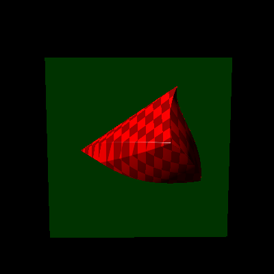
Experiment: 3d Visualization
Here are the two visualizers of neural networks I made for this post using WebGL2:
Neural Network Visualization 2D
Neural Network Visualization 3D
If you play around with this stuff and find anything interesting, please share!
