Bezier curves are pretty cool. They were invented in the 1950s by Pierre Bezier while he was working at the car company Renault. He created them as a succinct way of describing curves mathematically that could be shared easily with other people, or programmed into machines to make curves that matched the ones created by human designers.

I’m only going to go over bezier curves at the very high level, and give some links to html5 demos I’ve made to let you play around with them and understand how they work, so you too can implement them easily in your own software.

If you want more detailed information, I strongly recommend this book: Focus on Curves and Surfaces

Quadratic Bezier Curves

Quadratic bezier curves have 3 control points. The first control point is where the curve begins, the second control point is a true control point to influence the curve, and the third control point is where the curve ends. Click the image below to be taken to my quadratic bezier curve demo.

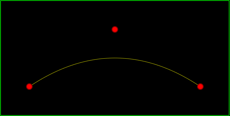
A quadratic bezier curve has the following parameters:

• t – the “time” parameter, this parameter goes from 0 to 1 to get the points of the curve.
• A – the first control point, which is also where the curve begins.
• B – the second control point.
• C – the third control point, which is also where the curve ends.

To calculate a point on the curve given those parameters, you just sum up the result of these 3 functions:

1. A * (1-t)^2
2. B * 2t(1-t)
3. C * t^2

In otherwords, the equation looks like this:

CurvePoint = A*(1-t)^2 + B*2t(1-t) + C*t^2

To make an entire curve, you would start with t=0 to get the starting point, t=1 to get the end point, and a bunch of values in between to get the points on the curve itself.

Cubic Bezier Curves

Cubic bezier curves have 4 control points. The first control point is where the curve begins, the second and third control points are true control point to influence the curve, and the fourth control point is where the curve ends. Click the image below to be taken to my cubic bezier curve demo.

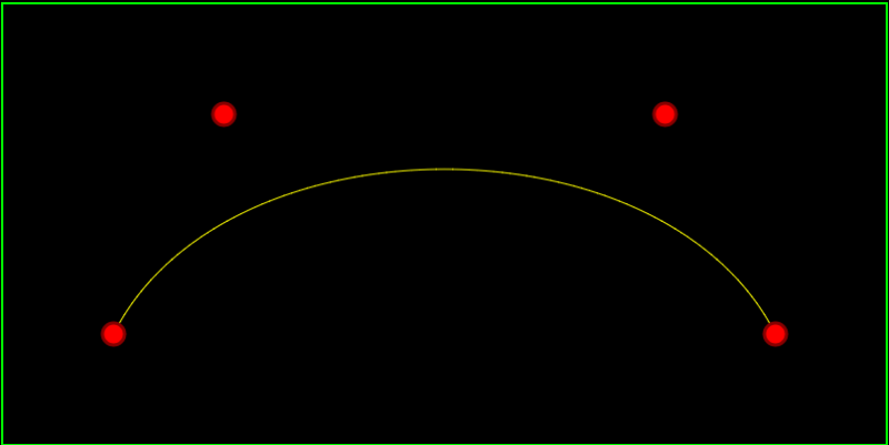
A cubic bezier curve has the following parameters:

• t – the “time” parameter, this parameter goes from 0 to 1 to get the points of the curve.
• A – the first control point, which is also where the curve begins.
• B – the second control point.
• C – the second control point.
• D – the fourth control point, which is also where the curve ends.

To calculate a point on the curve given those parameters, you just sum up the result of these 4 functions:

1. A * (1-t)^3
2. B * 3t(1-t)^2
3. C * 3t^2(1-t)
4. D * t^3

In otherwords, the equation looks like this:

CurvePoint = A*(1-t)^3 + B*3t(1-t)^2 + C*3t^2(1-t) + D*t^3

Math

You might think the math behind these curves has to be pretty complex and non intuitive but that is not the case at all – seriously! The curves are based entirely on linear interpolation.

Here are 2 ways you may have seen linear interpolation before.

1. value = min + percent * (max – min)
2. value = percent * max + (1 – percent) * min

We are going to use the 2nd form and replace “percent” with “t” but they have the same meaning.

Ok so considering quadratic bezier curves, we have 3 control points: A, B and C.

The formula for linearly interpolating between point A and B is this:
point = t * B + (1-t) * A

The formula for linearly interpolating between point B and C is this:
point = t * C + (1-t) * B

Now, here’s where the magic comes in. What’s the formula for interpolating between the AB formula and the BC formulas above? Well, let’s use the AB formula as min, and the BC formula as max. If you plug the formulas into the linear interpolation formula you get this:

point = t * (t * C + (1-t) * B) + (1-t) * (t * B + (1-t) * A)

if you expand that and simplify it you will end up with this equation:
point = A*(1-t)^2 + B*2t(1-t) + C*t^2

which as you may remember is the formula for a quadratic bezier curve. There you have it… a quadratic bezier curve is just a linear interpolation between 2 other linear interpolations.

Cubic bezier curves work in a similar way, there is just a 4th point to deal with.

Next Up

The demos above are in 2d, but you could easily move to 3d (or higher dimensions!) and use the same equations. Also, there are higher order bezier curves (more control points), but as you add control points, the computational complexity increases, so people usually stick to quadratic or cubic bezier curves, and just string them together. When you put curves end to end like that, they call it a spline.

Next up, be on the look out for posts and demos for b-splines and nurbs!