The last post talked about finite impulse response filters (FIRs) where the output of the filter was based on the current and previous input samples. (https://blog.demofox.org/2020/01/14/fir-audio-data-filters/)

In this post we are going to talk about infinite impulse response filters (IIRs) where the output of the filter is based not only on current and previous input samples, but also previous output samples.

This seemingly minor change makes for much more powerful and interesting filtering possibilities, but as it isn’t stateless, that means it must be evaluated serially (no SIMD!), and so is more computationally expensive.

The simple standalone C++ code that goes with this post is at: https://github.com/Atrix256/DSPIIR

The interactive web demo that goes with this post is at: http://demofox.org/DSPIIR/IIR.html

IIR Difference Equation

So let’s start with an order 2 FIR difference equation:

$y_n = a_0x_n + a_1x_{n-1} + a_2x_{n-2}$

Now let’s say we want the difference equation to include the previous two output samples too. We can just complete the pattern, by including some previous y terms with coefficient multipliers on the left side of the equation.

$y_n + b_1y_{n-1} + b_2y_{n-2} = a_0x_n + a_1x_{n-1} + a_2x_{n-2}$

We can then move everything but $y_n$ to the right side of the equation to get a function that gives us our current filtered output:

$y_n = a_0x_n + a_1x_{n-1} + a_2x_{n-2} - b_1y_{n-1} - b_2y_{n-2}$

You might be wondering why there is no $b_0$ term and the reason for that is because it would be a multiplier for $y_n$ which is weird. Do we really need to scale the output like that? Sometimes people will include the $b_0$ term, and will divide both sides of the equation by $b_0$ to get an equation like this:

$y_n = \frac{1}{b_0}(a_0x_n + a_1x_{n-1} + a_2x_{n-2} - b_1y_{n-1} - b_2y_{n-2})$

Let’s just pretend that if $b_0$ exists, it’s value is always 1, and then we can move on without it actually being there, complicating our equations needlessly.

So, to repeat it, here is a difference equation for an order 2 IIR filter, which is built on an order 2 FIR filter.

$y_n = a_0x_n + a_1x_{n-1} + a_2x_{n-2} - b_1y_{n-1} - b_2y_{n-2}$

You can pull out the $a_0$ parameter as a gain parameter again if you want to, but the b parameters don’t get the same sort of benefit, so you can leave them in their raw form.

$y_n = a_0(x_n + \alpha_1x_{n-1} + \alpha_2x_{n-2}) - b_1y_{n-1} - b_2y_{n-2}$

IIR Transfer Function

To calculate the transfer function, lets start back from where we added the previous outputs on the left side of the equation:

$y_n + b_1y_{n-1} + b_2y_{n-2} = a_0x_n + a_1x_{n-1} + a_2x_{n-2}$

Next, let’s take the z transform:

$y(z) + b_1y(z)z^{-1} + b_2y(z)z^{-2} = a_0x(z) + a_1x(z)z^{-1} + a_2x(z)z^{-2}$

We then factor out y(z) and x(z) to get:

$y(z)(1 + b_1z^{-1} + b_2z^{-2}) = x(z)(a_0 + a_1z^{-1} + a_2z^{-2})$

Since the transfer function is just y(z) divided by x(z) we can do simple algebra to do that now!

$\frac{y(z)}{x(z)}(1 + b_1z^{-1} + b_2z^{-2}) = a_0 + a_1z^{-1} + a_2z^{-2} \\ H(z) = \frac{y(z)}{x(z)} = \frac{a_0 + a_1z^{-1} + a_2z^{-2}}{1 + b_1z^{-1} + b_2z^{-2}}$

You can factor out the $a0$ term to be gain if you want, to get a more familiar looking top of the equation:

$H(z) = \frac{a_0(1 + \alpha_1z^{-1} + \alpha_2z^{-2})}{1 + b_1z^{-1} + b_2z^{-2}}$

From there you can plug in frequencies and see what sort of frequency and phase response you get, just like in the last blog post for FIRs.

You might notice that the transfer function is quadratic in the numerator, and the denominator. This is in fact called a “biquadratic filter” or a “biquad” for short.

Often times higher order filters (like EQs) are made by chaining multiple biquads together. Biquads are a pretty important staple of DSP.

Pole Zero Plot

You might wonder why in the last post we called it a “Pole Zero Plot” when there were zeros but no poles.

IIRs add poles to the pole zero plot and they are where the function shoots to infinity. This happens in a fraction when you divide by zero, so a pole is a place where the denominator of the transfer function is zero.

To make it explicit:

You solve the quadratic equation in the numerator to get the zeros of that quadratic equation, which are also the zeros of the filter.
You solve the quadratic equation in the denominator to get the zeros of that quadratic equation, which are the also the POLES of the filter.

That makes things pretty easy for making a pole zero plot. Calculating the zeros of the filter is the same, and you use the same technique to find the poles.

In the last post, we saw that the zeros of an order 2 FIR filter were at:

$z = \frac{-\alpha_1}{2} \pm \frac{\sqrt{\alpha_1^2-4\alpha_2}}{2}$

That still works for IIRS too. For poles, all you need to do is replace the alphas with bs:

$z = \frac{-b_1}{2} \pm \frac{\sqrt{b_1^2-4b_2}}{2}$

Example Filters

Unlike FIRs which are relatively tame and can only make certain frequencies lower, IIRs can cause frequency amplitudes to get much higher and even shoot off to infinity. That makes for some cool sounds by adding distortion to certain frequency notes of an instrument but not others.

Check the links section for the “RBJ cookbook” if you want to get deeper into the filters, but here are a couple interesting filters I found.

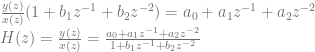
This one boosts low frequencies and attenuates high frequencies.

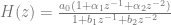
This does the reverse and boosts high frequencies while attenuating low frequencies.

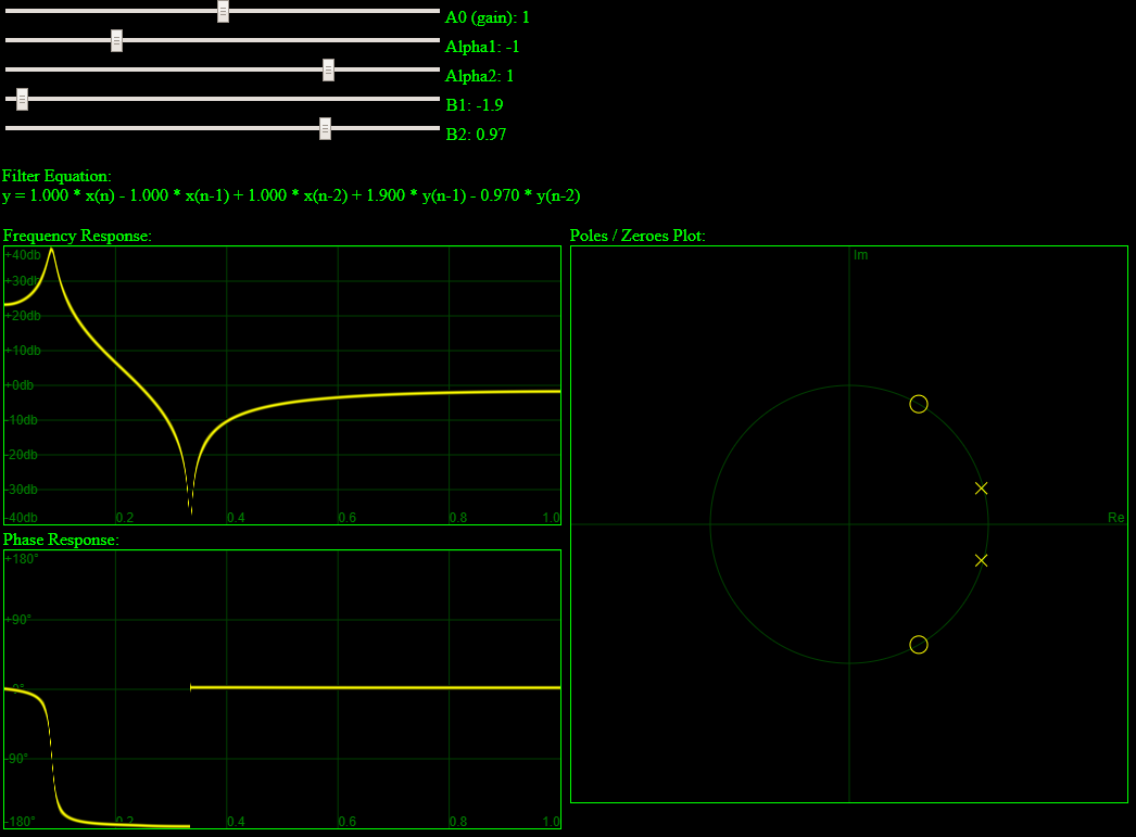
This makes use of both poles and zeros to make a really interesting sounding filter.

It’s also still fun to slowly move the controls back and forth while some simple instrumental loop plays. Filtering white noise is still really interesting too because white noise has all frequency content, which means filtering frequencies out or boosting them up will always affect white noise. That isn’t true of things with simpler frequency components. The extreme of this is the sine wave which only has a single frequency so is unaffected by other frequencies being boosted up or attenuated.

Crafting a Filter By Placing Zeros

Creating a biquad filter from zero and pole locations is pretty simple if you already can make an FIR filter by placing zeros. In fact, that is exactly how you place the zeros.

To place the poles, you do the exact same steps as placing the zeros, but the coefficients you get out are for b0, b1 and b2 instead of a0, a1 and a2.

Estimating Frequency Response From a Pole Zero Plot

Doing this from an FIR involved getting the distance from a point on the unit circle to every zero, multiplying all those distances together as a product and that is the amount the amplitude would be multiplied by.

Adding poles into the mix extends this.

As a second step, you get the distance from the point on the unit circle to every pole. You multiply all those pole distances together as a product and divide the previous product by this amount.

That’s all there is to it, and you should hopefully be able to see that this is why a frequency at the pole would shoot to infinity. The distance is zero so the frequency response shoots to infinity.

Oscillators

If you want to generate sinusoid waves of specific frequencies, you can use IIRs to do that by putting the poles on the unit circle, and leaving the zeros at the origin.

For a filter to be stable (not shoot off to infinity), the poles need to be inside of the unit circle, so putting them on the edge of the unit circle is playing with fire a bit, but the instability is also what makes the oscillator function.

We could talk about the algebra for calculating polynomials in the numerator and denominator of the transfer function to do this, but lets jump to the end and look at the simplified result of what to set the parameters to in the difference equation below:

$y_n = a_0x_n + a_1x_{n-1} + a_2x_{n-2} - b_1y_{n-1} - b_2y_{n-2}$

The parameters should be:

$a_0 = 1$
$a_1 = 0$
$a_2 = 0$
$b_1 = 2 cos(\omega)$
$b_2 = 1$

Where omega ( $\omega$ ) is the amount of radians to advance the wave form per sample.

If you plug these into the difference equation, you can simplify it to this:

$y_n = x_n - 2 cos(\omega)y_{n-1} - y_{n-2}$

These oscillators don’t need input and just want a steady stream of zeros. Because of this, we can remove the input from the equation.

$y_n = -2 cos(\omega)y_{n-1} - y_{n-2}$

The last thing you need to do however is to give it some initial starting state. If you make it so y[-1] and y[-2] are zero, to calculate y[0] and y[1], the oscillator won’t work correctly.

This is because we need to initialize the state (prior output) to be as if it’s been running all along.

So, you can set y[-1] to be $cos(-\omega*1)$ and y[-2] to be $cos(-\omega*2)$ . That will make it so the next sample will be $cos(0)$ which means the wave will start at zero degrees and continue.

You could initialize the state to whatever phase you wanted to, by initializing y[-1] and y[-2] to the prior two values to the desired phase.

As a quick and dumb example, let’s look at a sine wave that advances 180 degrees (pi radians) per sample. That means b1 will be 2, which makes our difference equation:

$y_n = -2y_{n-1} - y_{n-2}$

We’ll initialize y[-2] to be cos(-2pi) or 1, and we’ll initialize y[-1] to be cos(-pi) or 0.

Following the difference equation starting at y[0] we get…

$\begin{array}{|c|c|} \hline \text{y index} & \text{value} \\ \hline -2 & 1 \\ -1 & -1 \\ 0 & 1 \\ 1 & -1 \\ 2 & 1 \\ 3 & -1 \\ 4 & 1 \\ 5 & -1 \\ \hline \end{array}$

180 degrees is nyquist, and we can see that it’s doing the right thing of flipping between 1 and -1. It works with less clean numbers too, and the simple c++ code that goes with this post shows that working (https://github.com/Atrix256/DSPIIR).

Unfortunately, with less clean numbers, this method will start to drift from reality over time due to floating point imprecision. One way to deal with this is to reset the oscillator after every 360 degrees of advancement.

Nick Appleton (@nickappleton) has an alternate method if you are looking for a cheap oscillator.

First you make two complex numbers:

y = 1 + 0i
a = e^(i*omega)

Where omega is still the number of degrees the wave advances per sample. Another way to calculate a is: std::polar(1.0f, radiansPerSample)

Then, for each sample you do this:

y = y * a

the resulting complex number will have the cosine value in the real portion, and the sine value in the imaginary portion.

This has better numerical stability, which you can see in the c++ code output too.

Links

Here are some good links where i got info about oscillators.

http://dspfirst.gatech.edu/chapters/08feedbac/demos/recur/index.html

Click to access ece5655_chap8.pdf

There is a famous document called the “RBJ cookbook” which gives recipes for biquads that act in specific ways. RBJ stands for the author’s name Robert Bristow-Johnson. You can find it attached to the message at the link below!

https://www.musicdsp.org/en/latest/Filters/197-rbj-audio-eq-cookbook.html

Marc B Reynolds (@marc_b_reynolds) recently put out an interesting blog post talking about how it’s better to use integers to repeatedly add things (irrational numbers in his case) instead of using floats. There are some good lessons there that apply here as well I bet, probably especially for oscillators.

http://marc-b-reynolds.github.io/distribution/2020/01/24/Rank1Pre.html

The blog at the bottom of the sea

Programming, Graphics, Gamedev, Exotic Computation, Audio Synthesis

IIR Audio & Data Filters – Featuring Biquads

IIR Difference Equation

IIR Transfer Function

Pole Zero Plot

Example Filters

Crafting a Filter By Placing Zeros

Estimating Frequency Response From a Pole Zero Plot

Oscillators

Links

Leave a Reply Cancel reply

IIR Difference Equation

IIR Transfer Function

Pole Zero Plot

Example Filters

Crafting a Filter By Placing Zeros

Estimating Frequency Response From a Pole Zero Plot

Oscillators

Links

Share this:

Like this:

Related

Leave a Reply Cancel reply