About 6 years ago I wrote about how to fit curves, surfaces, volumes, and hypervolumes to data points in an “online algorithm” version of least squares – that is, you could update the fit as new data points come in.

Incremental Least Squares Curve Fitting

Incremental Least Squares Surface and Hyper-Volume Fitting

In this post, I’m going to show how to adjust the least squares equations to be able to give weights for how important data points are in the fit. We’ll be looking at curves only, and not focusing on the “online algorithm” aspect, but this will work for both surfaces/volumes as well as the online updating.

The simple standalone C++ code that goes with this post can be found at https://github.com/Atrix256/WeightedLeastSquares

If you google weighted least squares, or look for it on youtube, almost every example you are likely to find talks about it being used when the variance of data points are different in different parts of the graph, and that is used to make points contribute more or less to the final fit.

That is a pretty neat usage case, but if you are just trying to fit a curve to data points as a way to compress data or optimize calculations, you probably are not really concerned with the variance of the data points you are trying to fit. Luckily, weighting data points in least squares is pretty simple.

Here is the equation you solve in ordinary least squares (OLS):

where A is a matrix that contains all the powers of x of each data point, y is a vector that contains the y values of each data point, and x is polynomial coefficients that we are trying to solve for.

A pretty straightforward way to solve this equation for x is to make an augmented matrix where the left side is , and the right side is .

From there you can do Gauss-Jordan elimination to solve for x (https://blog.demofox.org/2017/04/10/solving-n-equations-and-n-unknowns-the-fine-print-gauss-jordan-elimination/). At the end, the left side matrix will be the identity matrix, and the right side vector will be the value for x.

Adjusting this formula for weighting involves introducing a weight matrix called W. W has a zero in every element, except along the main diagonal where the weights of each data point are. .

There is something called “generalized least squares” (GLS) where the weight matrix is a covariance matrix, allowing more complex correlations to be expressed with non zeroes off of the main diagonal, but for weighted least squares, the main diagonal gets the weights of the data points.

The equation to solve for weighted least squares (WLS) becomes this:

You can make an augmented matrix like before:

And use Gauss-Jordan elimination again to solve for x:

Examples

Here are a few runs of the program which again is at https://github.com/Atrix256/WeightedLeastSquares

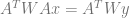
Starting with 3 data points (0,0) (1,10), (2,2) all with the same weighting, we fit them with a line and get . It’s interesting to see that data points 0 and 2 each have an error of +3 while data point 1 has an error of -6.

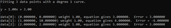
If we set the weighting of the 2nd point to 0.0001, we can see that it absorbs most of the error, because the weighting says that it is 10,000 times less important than the other data points.

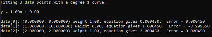
Alternately, we can give it a weight of 10.0 to make it ten times as important as the other two data points. The error becomes a lot smaller for that data point due to it being more important.

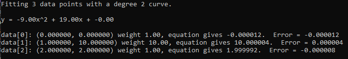
If we switch to a quadratic curve, all three points can be well fit, with the same weights.

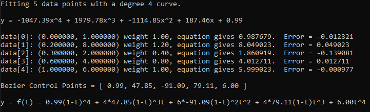
The example code works in any degree and also shows how to convert from these power basis polynomials to Bernstein basis polynomials, which are otherwise known as Bezier curve control points (more info on that here: https://blog.demofox.org/2016/12/08/evaluating-polynomials-with-the-gpu-texture-sampler/). The weighting you see in curves is not the same as the weighting here. When you convert the polynomial to a Bezier curve, it’s an unweighted curve. Weighted Bezier curves are made by dividing one Bezier curve by another and are called “Rational” curves, where unweighted curves are called “Integral” curves. Rational (weighted) curves are able to express more shapes than integral curves can, even when those integral curves are made by weighted least squares.

Closing

While we used weighted least squares to give different weightings to different data points, the main motivation you find on the internet seems to be about having different levels of confidence in the data points you get. This makes me wonder if we could use this in graphics, using 1/PDF(x) as the weighting in the least squares fitting like we do in importance sampled monte carlo integration. This seems especially useful if using this as an “online algorithm” that was improving a fit as it got more samples, either spatially or temporally.