I recently wrote a blog post that shows how interleaved gradient noise is a low discrepancy grid optimized for the 3×3 neighborhood sampling you find in temporal anti aliasing (TAA): https://blog.demofox.org/2022/01/01/interleaved-gradient-noise-a-different-kind-of-low-discrepancy-sequence/

In some TAA implementations, instead of taking the full 3×3 neighborhood around a pixel, only the 4 cardinal direction neighbors will be sampled, making a plus shape (+) of sampling. This can reduce memory bandwidth requirements because it cuts the neighborhood sampling in half, from 8 samples down to 4.

In this post I’ll show a low discrepancy grid that is optimized for this sampling pattern. The formula for it is below, where pixelX and pixelY are integer pixel coordinates.

z = ((x+3y+0.5)/5) mod 1

or as code:

float PlusShapedLDG(int pixelX, int pixelY)
{
    return fmodf((float(pixelX)+3.0f*float(pixelY)+0.5f)/5.0f, 1.0f);
}

While we are talking about LDGs I also want to show another one based on a generalization of the golden ratio to 2D, made by Martin Roberts (https://twitter.com/TechSparx) which is calculated like this:

z = (x / 1.32471795724474602596 + y / (1.32471795724474602596 * 1.32471795724474602596)) mod 1

or as code:

float R2LDG(int pixelX, int pixelY)
{
    static const float g = 1.32471795724474602596f;
    static const float a1 = 1/g;
    static const float a2 = 1/(g*g);
    return fmodf(float(pixelX)*a1+float(pixelY)*a2, 1.0f);
}

At the end of the post we’ll analyze these noise types along with some others:

Derivation of Plus Shaped Low Discrepancy Grid

It took a couple attempts at deriving this before I was successful.

We want a regular grid of values where each plus shape has every value 0/5, 1/5, 2/5, 3/5, 4/5. When I say every plus shape, I’m including overlapping ones. In TAA when a pixel looks at it’s plus shaped neighborhood, we want it to get an accurate as possible representation of the total possibilities for that pixel in that region of the screen. The pixels it finds should very accurately represent the actual histogram of what is possible in this area of pixels. The more accurate we make this, the better the neighborhood sampling history rejection/preservation logic will work.

I started out by putting symbols in a plus shape like this, planning to solve for the actual values later:

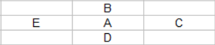
I next needed to figure out how to fill in the corners of these pixels. I opted to do so like this, trying to make the repeated values be as far away from the original values as possible.

You can see that at the center of each edge is the center of a plus shaped pattern which has 4 of the 5 letters already, so we can complete the plus by adding the 5th letter.

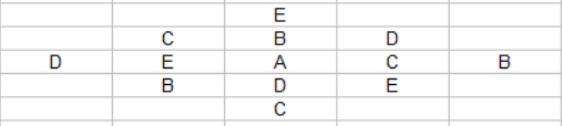
To fill out the rest of this grid, you can notice that there is a pattern of how letters are duplicated in the above: Their copy is either two to the right and one down, or two down and one to the left. You can use this pattern to complete this 5×5 square.

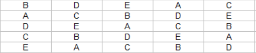
After filling out this 5×5 square you can see that both rules are true: symbols are repeated both two cells down one cell to the left, and also two cells to the right and one cell down.

Interestingly, if you continue growing this square outwards, it just repeats this 5×5 tile over and over, so we are done figuring out how to tile our values, but we still don’t know where the values should be or how to make a formula that calculates them.

At first I tried plugging in 0.0 for A, 0.2 for B, 0.4 for C, 0.6 for D and 0.8 for E. That made a really messy looking grid that I was unsure how to replicate with a formula.

Thinking about it differently, I looked at the first row which goes in order B,D,E,A,C and I made the values be in that order. B got value 0.0, D got 0.2, etc. That left me with this:

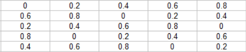
To make things easier to see, here are those values multiplied by 5:

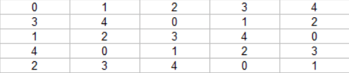
It’s a bit easier to see a pattern here, isn’t it?

Starting at the upper left as (0,0), we can see that going to the right, the value increases by 1. Since this tile repeats infinitely, it means that when we go past 4, we go back to zero. So for that the formula would be z = x % 5.

We can also notice that taking a step down on the y axis, we add 3, but once again wrap around if we get past four. Putting this into the previous equation, it becomes z = (x + 3y) % 5.

We want this divided by 5 to be the values 0/5, 1/5, … 4/5, so our final equation becomes z = Fract((x + 3y)/5). Or z = ((x + 3y)/5) mod 1. Whichever notation you prefer.

Now for some subtlety. If you take the average of 0/5, 1/5, 2/5, 3/5, 4/5 you get 0.4. To make this unbiased, we want the average to be 0.5, which we can do by adding 1/10th to every value. That means our equation becomes z = (((x + 3y)/5) + 1/10) mod 1 or z = ((x + 3y + 0.5)/5) mod 1.

Another way to solve this problem could be instead of having values 0/5, 1/5, 2/5, 3/5, 4/5, you could instead divide by 4 to get 0/4, 1/4, 2/4, 3/4, 4/4, which would average to 0.5 as well. You may very well want to do that situationally, depending on what you are using the numbers for. A reason NOT to do that though would be in situations where a value of 0 was the same as a value of 1, like if you were multiplying the value by 2*pi and using it as a rotation. In that situation, 0 degrees would occur twice as often as the other values and add bias that way, where if you were using it for a stochastic alpha test, it would not introduce bias to have both 0 and 1 values.

Before analyzing this noise, let’s talk about the R2 LDG.

R2 Low Discrepancy Grid

The R2 low discrepancy grid was made by Martin Roberts and is based on his R2 low discrepancy sequence which generalizes the golden ratio to 2D (http://extremelearning.com.au/unreasonable-effectiveness-of-quasirandom-sequences/).

To make the R2 low discrepancy sequence, you divide the index by 1.32471795724474602596 and fract to get the x component of the LDS, and divide index by 1.32471795724474602596 * 1.32471795724474602596 and fract to get the y component of the LDS.

To make the R2 low discrepancy grid, you divide the integer x pixel coordinate by 1.32471795724474602596, divide the integer y pixel coordinate by 1.32471795724474602596*1.32471795724474602596, add them together and fract to get the final scalar value.

Interestingly, this works with any rank 1 lattice, so there is some exploration to be done here IMO, to find more low discrepancy grids and see what sort of properties they have.

In fact, you can express both the plus shaped LDG and this R2 LDG in this rank 1 lattice style LDG:

z = (x * A + y * B) mod 1

With the plus shaped LDG, A is 1/5 and B is 3/5.

With the R2 LDG, A is 1 / 1.32471795724474602596, and B is 1 / (1.32471795724474602596*1.32471795724474602596).

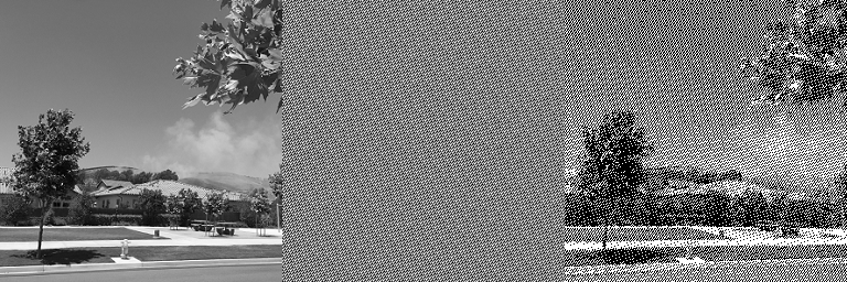
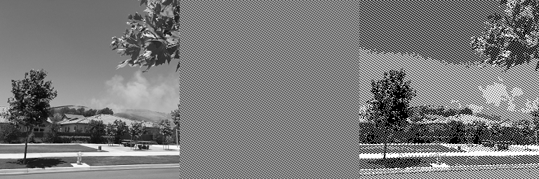
Stippling

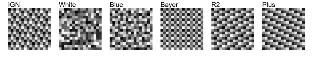
Here we’ll use various types of grid noises to turn greyscale images into black and white stippled images. We do this by testing each image pixel against the corresponding noise pixel. If the noise pixel is a lower value (darker) than the image pixel, we put a black pixel in the output, else we put a white pixel in the output.

White Noise

Blue Noise

Bayer

IGN

R2

Plus

Stochastic Transparency

Here we test noise values against the transparency value and if the noise is less, we write a magenta pixel, else we don’t. The percentage of pixels that survive the transparency test are shown, and ideally would match the transparency value for the best results.

10%

20%

30%

40%

One thing worth talking about is that the percentage of white noise pixels that survive the alpha test swings pretty wildly compared to what the actual transparency value is. This effectively makes the pixels more opaque or more transparent than they should be, which causes problems when filtering spatially and/or temporally. That is on top of how white noise clumps together and leaves holes, which make it harder to filter than more equally spaced data points.

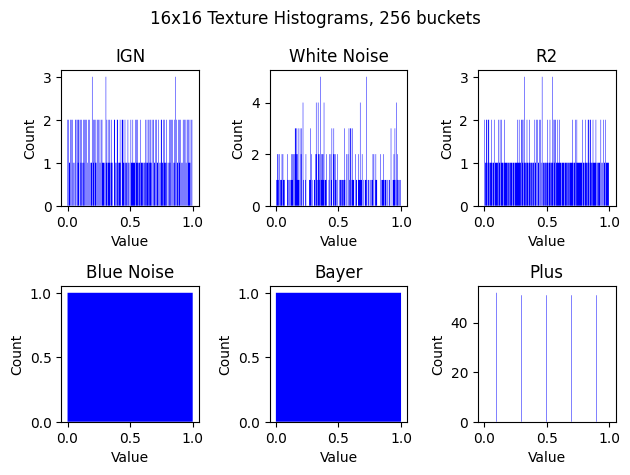
Another thing worth pointing out is that the plus shaped noise is VERY wrong at 10% and 30% percent, but does very well at 20% and 40%. The reason for this is because of how the plus noise is discretized into 1/5th increments. The other noises have all values (0 to 255, because these are U8 textures) which means they work better at arbitrary opacities.

With all noises except the plus noise, as you smoothly increase the opacity, pixels will slowly start appearing. With the plus noise, as you smoothly increase the opacity, pixels will appear in large clumps, instead of appearing one by one. A way to deal with this could be to take a hint from stratified sampling, and instead of adding 1/10th to the noise to unbias it, you instead add a random number between 0 and 1/5th. It will still have the correct average, so won’t be biased, but the random numbers could break things up a bit. You could even use a blue noise texture as the source of those random numbers perhaps.

Here is a histogram of each noise, which shows what I’m talking about regarding the plus noise:

3×3 Region Analysis

I’ll only include IGN and the new ones. The rest of them can be found in the IGN LDG blog post at https://blog.demofox.org/2022/01/01/interleaved-gradient-noise-a-different-kind-of-low-discrepancy-sequence/

IGN

Plus

R2

The plus shaped noise does very poorly in these 3×3 regions, because there are only 5 possible values, and we are looking at how unique the values are from 9 different pixels. It definitely is not optimized for this usage case.

R2 does quite a bit better, but not as good as IGN, which makes sense because R2 is meant for “general purpose use” as a low discrepancy grid, where IGN is meant specifically to have great LDS properties in a 3×3 region.

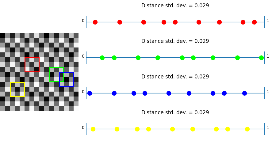
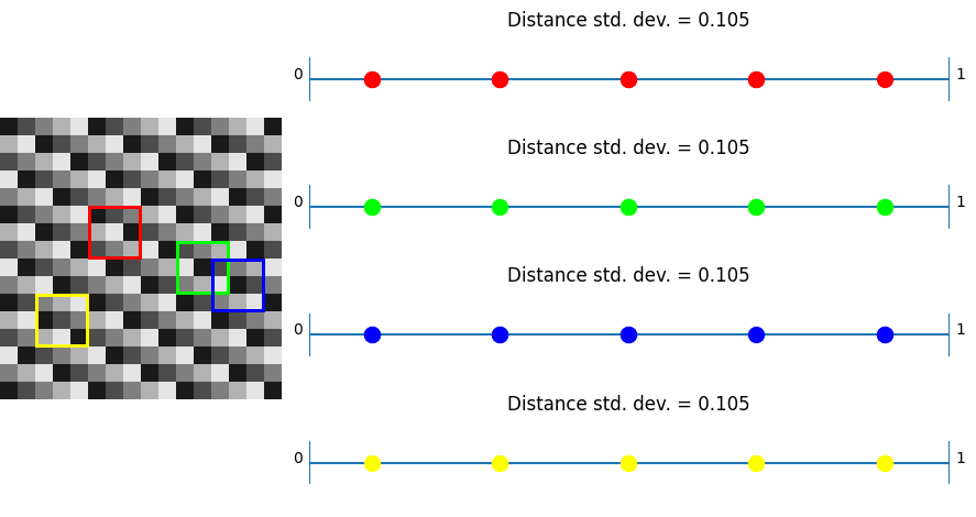
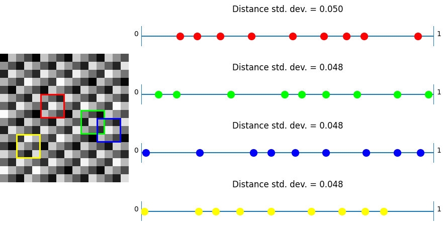
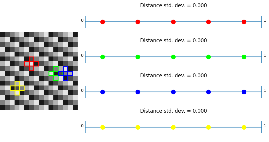
Plus Shaped Region Analysis

White

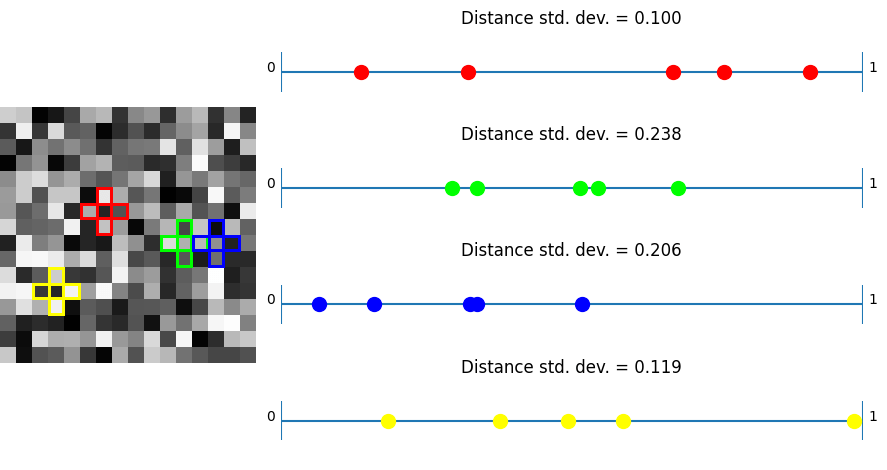
Blue

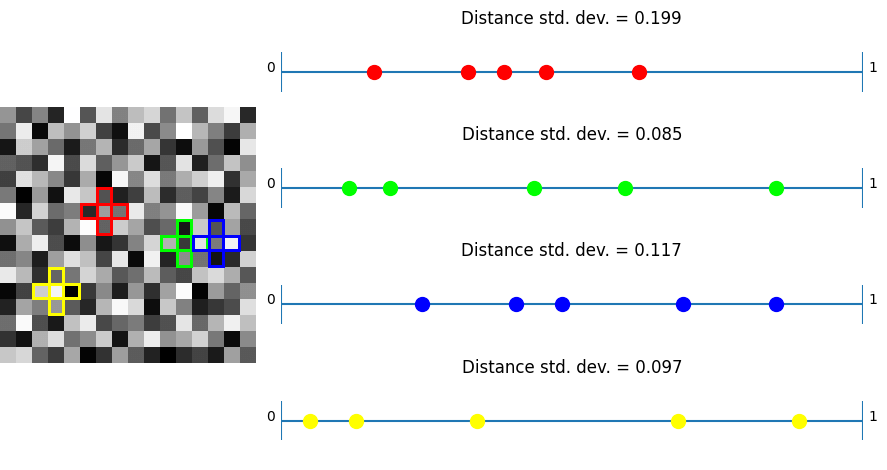
Bayer

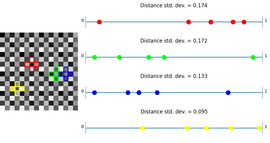
IGN

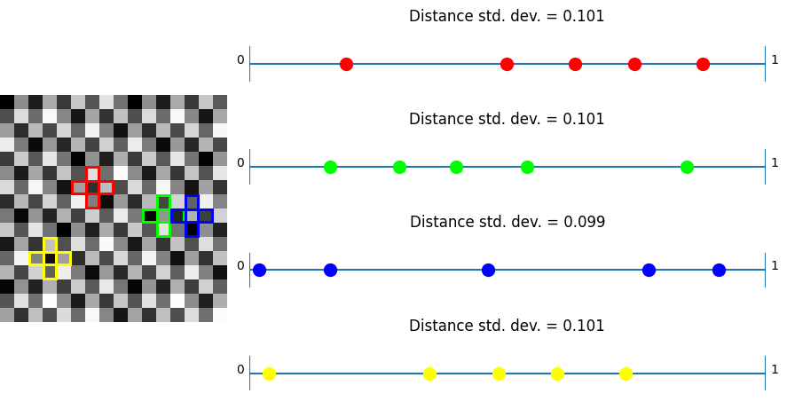
R2

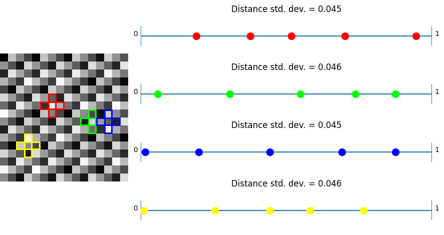
Plus

In this test, taking plus shaped samples and analyzing how their values lie on a numberlines, white noise shows the worst results as per usual. Bayer and also blue noise don’t do that great either.

Now, unlike the last test, where IGN beat R2, we can see that R2 beats IGN. This shows again that R2 is good in “general purpose uses” where IGN is optimized towards just 3×3 blocks.

Lastly, we see the plus noise doing the best here – in the situation it was optimized for, which is no surprise. Any randomization added to this noise to help break up the quantization artifacts will make this specific test have a higher standard deviation of distances. With good noise (like blue noise?) used to jitter, the standard deviation may only go up a little. Having the standard deviation go up a little bit probably would help results in general when using this noise. After all, the goal of low discrepancy sequences is to have LOW discrepancy (discrepancy being some variance in the spacing here) but not NO discrepancy, since having no discrepancy is regularly spaced sampling, which has some bad properties, including aliasing.

Plus Shaped Noise vs IGN

Jorge (maker of IGN) derived the same plus shaped sampling noise that I did (I did my derivation after he said he had found such a noise, and then we compared to see if we found the same thing). He put the noise through some tests, using a plus shaped neighborhood sampling TAA implementation and he found that IGN performed better than this plus shaped sampling noise. I’m not sure the details of his test, or how much better IGN did, but it would be interesting to do some analysis and share those details. I may do that at some point, but if someone else does it first, please share! I’m curious if the problems came up due to the discretized values of this plus noise, and if jittering the values using good noise helps the problems at all.

You might be wondering how IGN is fully floating point when the plus noise is discretized.

If we tried to derive IGN the same way as we did with the plus noise, you would want to make every 3×3 block of pixels to have every value 0/9, 1/9, … 8/9, even overlapping ones. If you work through this generalized sudoku, you’ll find that there are too many constraints and it actually isn’t solvable. A way to get around this is to have some numerical drift of the values over space, so that you spread the error of it not being solvable over distance. That is what IGN does and is why it isn’t a discretized noise, having only x/9 values. I’m not sure if IGN optimally distributes this error evenly over distance or not though. That would be an interesting thing to look at.

Closing

Hopefully you found this post interesting and have some new tools in your toolbelt.

If you ever need VECTOR valued noise but only have SCALAR valued noise, you can try putting your scalar values through a Hilbert curve to turn your scalars into vectors. In my experience, this isn’t as high quality as having true vector valued noise, but does actually work in preserving the scalar noise properties in the resulting vector valued noise somewhat so is a lot better than nothing.

If you try using this noise or try out any of the things mentioned above or similar, it would be great to hear how it goes for you, either here as a comment or on twitter at https://twitter.com/Atrix256.

Thanks for reading!