This goes along with the blog post for generating blue noise point sets using sliced optimal transport at https://blog.demofox.org/2023/12/24/making-blue-noise-point-sets-with-sliced-optimal-transport/

The code implementing this can be found on github at https://github.com/Atrix256/SOTPointSets/blob/main/squarecdf.h

The diagrams in this post were made at https://www.geogebra.org/geometry

I tried deriving this a few times, but kept getting a PDF that was more complex than I’d like. It turned out my mathematically inclined friend, and frequent co-author William Donnelly (such as in https://www.ea.com/seed/news/constant-time-stateless-shuffling), had already worked this out previously, so he shared how he did it, which I explain below more as a sketch than a proof. Treat the code as the source of truth here 🙂

The PDF

Let’s start out with a square centered at (0,0) with a width and height of 1.

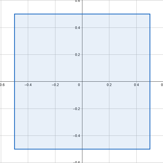
Now we rotate it. This is 25 degrees, but the specific angle doesn’t matter.

We want to find the height of the shaded region at a given point x. For now we’ll stick to the right half of the rotated square. In the diagram below, we are trying to find the length of the line segment EF. This is also the hypotenuse of the right triangle EFG.

The definition of cosine of theta is that it’s “adjacent over hypotenuse”, or the length of EG over the length of EF. We know that the length of EG is 1 because that is the height of the square, so we have:

We can re-arrange that to get:

Theta () is the angle that our square is rotated by.

That is our formula for the height of the rotated square at a point x, and it is a constant value from x=0 to the x value of P.

The value of P before rotation is (0.5, 0.5). The 2d rotation formula is:

So, the x value of P after rotation is . This is the point at which our height equation needs to change to a different formula.

While we are rotating points, we can also rotate the point Q (0.5, -0.5) and get an x value of .

That x value of Q is where our projected height goes to 0, and at the x value of P, we know the projected height is . We also know that the area is a linear function (it’s the top line minus the bottom line). So, to get the 2nd part of our height function, we are trying to find the formula of the second between P and Q below:

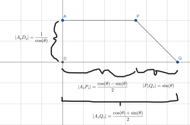
We know that the distance from P to Q on the x axis is the x axis point of Q minus the x axis point of P.

We know the height already because it’s the same as the distance for AD, so the slope of the line from P to Q is rise over run, or:

instead of making a formula from P and subtracting the slope, we can instead subtract x from the maximum value x can take, and multiple the slope in. We know that Q is 0, so that is our formula:

We now have a piecewise height function, for the right side of the x axis, for a rotated square:

The sines and cosines make the formula look complex, but f your equation is passed the normalized vector that the points are being projected onto, the x axis is cosine of theta and the y axis is the sine of theta. That is point F below.

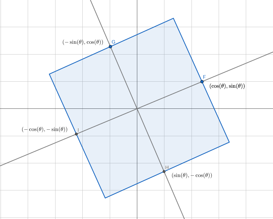
Due to vertical and horizontal symmetry of the rotated square, we can take the absolute value of that vector’s components to bring it to the 1st quadrant. We can go further and set cosine to the maximum of x and y, and sine to the minimum of x and y, and bring the solution to 0 to 45 degrees.

float cosTheta = std::max(std::abs(direction.x), std::abs(direction.y));
float sinTheta = std::min(std::abs(direction.x), std::abs(direction.y));

Doing that, our height function handles all possible angles. Also, because the area of our square is 1 – it is centered at (0,0) with a width and height of 1 – our height function is a normalized PDF!

The CDF

Next we need to integrate the PDF into a CDF. The first section of the piecewise PDF is constant so when integrated will become linear. The second section is linear so will become quadratic.

That gives us:

Will has the CDF’s values centered at 0, so subtracts the second case from 0.5 and returns the negated version of it if x < 0, else returns the positive version.

The Inverse CDF

The linear section of the CDF is easy enough to invert:

We need to know what y value switches from this linear section to the quadratic section though. For that, we can plug the maximum value of that PDF section into that section of the PDF to get that y value.

So, we have the first section of our inverse CDF. For the second half, I’ll wave my hands here a bit and give the answer. Keep in mind, this is for a “CDF” with y values ranging between -0.5 and 0.5. You can shift the result if you need a more traditional CDF.

The Code

It’s on github, but also pasted here in case that link is dead in the future for some reason.

// Derived By William Donnelly

struct float2
{
	float x, y;
};

// The square is centered at (0,0) and has width and height of 1.
// So, the square is (x,y) in (-0.5,0.5)^2
// The CDF / ICDF are then shiften to be between -0.5 and 0.5, instead of being from 0 to 1.
namespace Square
{
	inline float InverseCDF(float u, float2 d)
	{
		float c = std::max(std::abs(d.x), std::abs(d.y));
		float s = std::min(std::abs(d.x), std::abs(d.y));

		if (2 * c * std::abs(u) < c - s)
		{
			return c * u;
		}
		else
		{
			float t = 0.5f * (c + s) - sqrtf(2.0f * s * c * (0.5f - std::abs(u)));
			return (u < 0) ? -t : t;
		}
	}

	inline float CDF(float x, float2 d)
	{
		float c = std::max(std::abs(d.x), std::abs(d.y));
		float s = std::min(std::abs(d.x), std::abs(d.y));

		if (std::abs(x) > 0.5 * (c + s))
		{
			return (x < 0.0f) ? -0.5f : 0.5f;
		}
		else if (std::abs(x) < 0.5f * (c - s))
		{
			return x / c;
		}
		else
		{
			float fromEnd = (0.5f * (c + s) - std::abs(x));
			float u = 0.5f - 0.5f * fromEnd * fromEnd / (c * s);
			return (x < 0.0f) ? -u : u;
		}
	}

	inline float PDF(float x, float2 d)
	{
		float c = std::max(std::abs(d.x), std::abs(d.y));
		float s = std::min(std::abs(d.x), std::abs(d.y));

		if (abs(x) < 0.5f * (c - s))
		{
			return 1 / c;
		}
		else if (abs(x) < 0.5f * (c + s))
		{
			float fromEnd = (0.5f * (c + s) - std::abs(x));
			return fromEnd / (c * s);
		}
		else
		{
			return 0.0f;
		}
	}
};