This post goes through a common exercise in applying optimal transport to graphics, using informal language and simple, standalone C++ to implement it. The post uses sliced optimal transport which compared to standard optimal transport solvers is more intuitive, more efficient, and makes for a simpler implementation.

The code that goes with this post is ~300 lines of c++ code that uses STB for image reading and writing, but is otherwise standalone, and can be found at https://github.com/Atrix256/SOTImageColors.

Optimal Transport

The diagram below shows a number of doughnuts at 3 bakeries, that need to go to 5 cafes. The supply (blue numbers) equals the demand (green numbers), for 13 doughnuts total that need to be transported from bakeries to cafes.

Optimal transport is the answer to the question “How many baked goods should each bakery send to each restaurant to minimize the delivery distance (cost)?”.

Solving this problem in general is pretty complex and computationally costly. Check out the Sinkhorn Algorithm and Hungarian Algorithm for details.

The problem becomes a lot simpler in 1 dimension though. You sort the bakeries by x, and the cafes by x, then assign deliveries by matching index. The first bakery delivers to the first cafe, the second bakery delivers to the second cafe and so on.

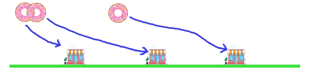
In this diagram, each bakery only has 1 doughnut, and each cafe only wants 1 doughnut. To make a bakery have more than 1 doughnut, you would just duplicate the bakery to make N in the same location, for the N doughnuts produced. To make a cafe want more than 1 doughnut, you would similarly duplicate the cafe to make M in the same location, for the M doughnuts required. The algorithm is the same and is solved by just sorting both lists!

Sliced Optimal Transport

Sliced optimal transport is a magical algorithm that it lets you solve higher dimensional optimal transport problems by solving several one dimensional optimal transport problems instead.

More specifically, you generate a uniform random unit vector, project your source and target data onto that vector using dot product, and sort, which makes the points equally spaced along the line.

Doing that once isn’t going to be enough to solve for the optimal transport, so you do that several times with different uniform random vectors, in a batch, and keep an average of the full N dimensional vector that each projection moved each point. At the end of the batch, you move the source towards the destination by that amount.

Doing one batch isn’t going to be enough to solve for the optimal transport either, so you do several batches, until it converges to an answer.

The number of vector projections per batch, and the number of batches, are hyperparameters that you need to tune for your particular optimal transport problem. You could also set up heuristics, like ending the program when the total amount of movement was below a certain threshold.

If you sat down to implement this, you might wonder how to generate an N dimensional uniform random unit vector, where N is any number of dimensions. Luckily there is a really nice and simple way. You generate an N dimensional vector using a normal distribution for each vector component, then normalize it! std::normal_distribution is your friend, in C++.

Interpolating Color Image Histograms

The goal of this post is to have one image take the colors of another image, which you may know as “Color Grading” if you work in games or graphics.

How does this relate to optimal transport, and our bakeries and cafes?

Each pixel in our source image is a bakery with one doughnut. The RGB value of the pixel is the location of that bakery in a 3D space, if we treat RGB as XYZ for a 3 dimensional vector.

Each pixel in the image we want to take the colors of is a cafe that wants one doughnut. The RGB value of the pixel is the location of that cafe in a 3D space as well.

Our goal is to move each source image pixel RGB value (each doughnut) to a target color image pixel RGB value (a cafe). In the end, there will only be the colors from the target color image.

We could just do this randomly, and set each source color image pixel to a randomly selected target color image pixel, but the source image would look like random noise.

If we do this using optimal transport instead, it means that we assign target color image pixel colors to source image pixels such that we’ve modified the source image pixels the least. That means the relationship between pixels will largely stay the same and we will end up with something that still looks like our source image, but uses only the colors from the target color image.

Note: the source image and the target color image need to be the same size, so that the number of doughnuts available from the bakeries match the number of doughnuts desired at the cafes.

Algorithmic Details

I didn’t spend very long tuning the batch size and number of iterations, but I found good results with a batch size of 16 and 100 iterations.

The sorting is the bottleneck by far, but I found that each batch could be done in parallel, which helped performance a lot on my machine.

The images I used were 792×516 and I am able to calculate optimal transport for color histograms in about 16 seconds on my machine.

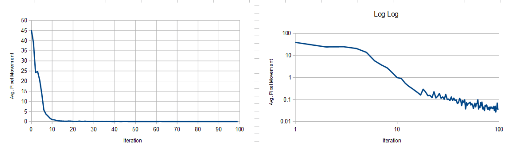
I had the algorithm spit out the average movement per pixel to a csv after every step, with the assumption that smaller steps mean it is closer to convergence. Below is the graph of “big cat”, but the other two were very similar.

Images

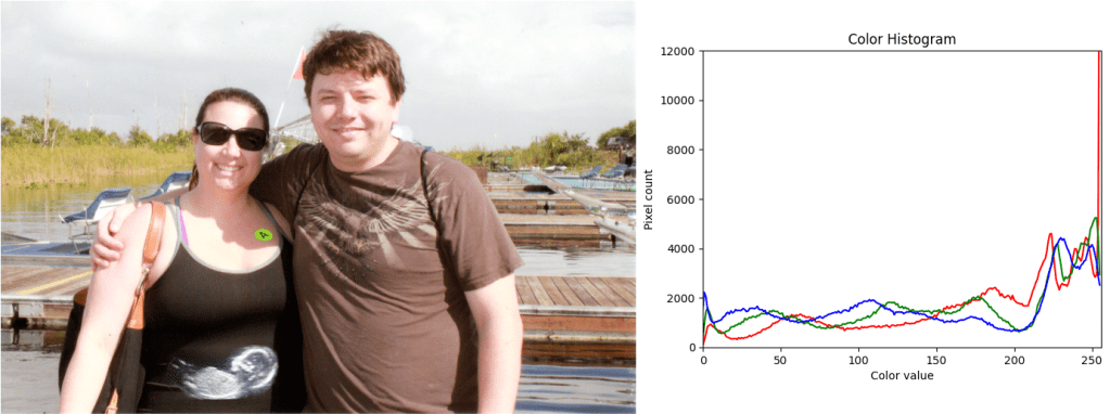
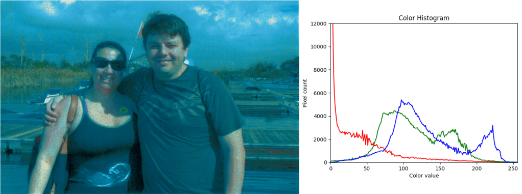
Here is the source image I used (florida), and it’s histogram.

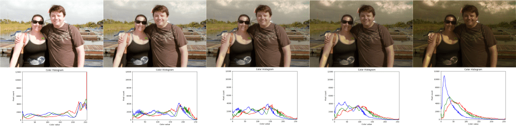
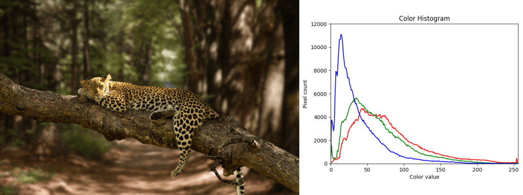
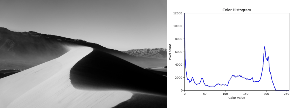
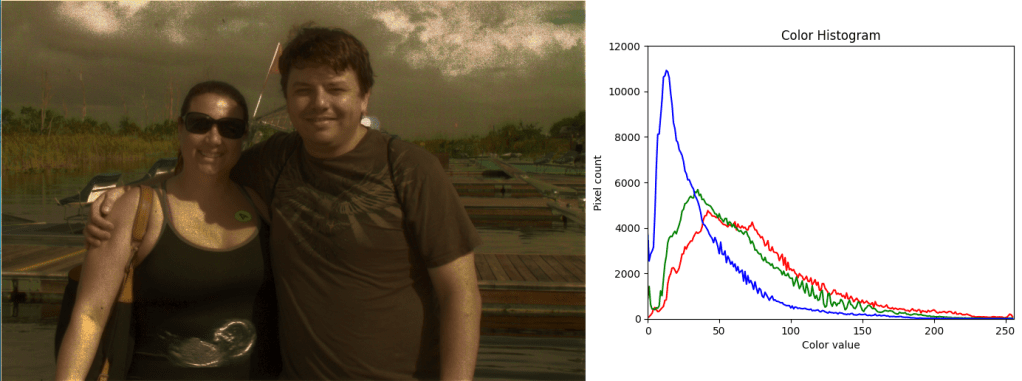
Here are the 3 images i used as targets, along with their histograms: bigcat, dunes, turtle.

Results

Florida remapped to big cat

Florida remapped to dunes

Florida remapped to turtle

If you compare the histograms closely, you’ll see that while they are not a 100% match, they are extremely close. Below shows the difference between the big cat histogram and the florida remapped to big cat histogram.

This is also noticeable in the dunes result, where the histogram shows that the colors are not all perfectly grey. An easy way to compare is to open one of the source image/histograms in the last section in one browser tab, and the corresponding result below in another tab, and flip back and forth.

Interpolation

Solving the optimal transport problem tells you where to move each source image pixel to make the color histogram match a target. Instead of moving the pixels all the way in the RGB 3d cube to the correct location, you can move the pixels part of the way there, thus interpolating the source image histogram to the target image histogram. Below shows an interpolation from florida to big cat, at 0%, 25%, 50%, 75% and then 100%.

When you interpolate from A to B by 25%, you are really doing barycentric interpolation along a line (a 1D simplex) with barycentric coordinates (u,v) = (0.75, 0.25). To get the result, you are multiplying the original image by 0.75, the target image by 0.25, and adding the results together.

Barycentric interpolation generalizes to any dimension. In 2D, you get three barycentric coordinates and are interpolating on a triangle.

Also, while barycentric coordinates are meant for doing interpolation, but having all coordinates sum up to 1, and all be between 0 and 1, you can break those assumptions. When a coordinate is less than 0 or greater than 1, then you are doing barycentric extrapolation. You could do the same here, if you for instance just wanted a photo to be LESS like another photo, as far as the color histogram was concerned.

I’ll leave that to you to experiment with though, if that sounds interesting 🙂

Lastly, the code uses white noise uniform random lines to project onto. White noise is good “at the limit” but for smaller numbers of samples, it tends to clump up and leave holes. I’m betting that using a low discrepancy sequence to generate the lines would give better results that converge faster. I’m leaving that as a teaser for you again, but also think I will give that a try in the future.

Links and Resources

Here’s a post very similar to mine, also in C++: https://dcoeurjo.github.io/OTColorTransfer/

A previous blog post of mine talked about how to use optimal transport to measure the similarity of two 1D histograms. Check it out here: https://blog.demofox.org/2022/07/27/calculating-the-similarity-of-histograms-or-pdfs-using-the-p-wasserstein-distance/

A simple introduction on Sinkhorn distances: https://amsword.medium.com/a-simple-introduction-on-sinkhorn-distances-d01a4ef4f085

Sliced Optimal Transport: https://www.numerical-tours.com/matlab/optimaltransp_4_matching_sliced/