January « 2025 « The blog at the bottom of the sea

I stumbled across a very cool YouTube video today that talks about how to look for alternate ways of labeling sides of two dice to give you the same random number distribution as if you added two standard dice together. https://www.youtube.com/watch?v=xVRRykIyll0

Making customized dice give desired probability distributions is an interesting topic (like for game design!), but the math that was used in the video was also pretty neat. I’ll walk you through what they did and then we can talk about why it works, from two different points of view.

(I’m going to refer to a single die as “a dice”, apologies in advance!)

The Problem Statement

If you roll a single dice, the probability of getting each possible value is the same: 16.666…%.

However, if you roll two dice and add them together, the probability of getting each possible value is not equal. You can only get a two by rolling a 1 and a 1, but you can roll a four by rolling a 1 and a 3, a 2 and a 2, or a 3 and a 1. There is only one way to roll a two, but there are three ways to roll a four. So, rolling a four is three times more likely than rolling a two. The probability for each possible value is described by the binomial probability distribution below.

Dice Sum	# Of Ways	Probability (Rounded)	Dice Values
2	1	3%	11
3	2	6%	12, 21
4	3	8%	13, 22, 31
5	4	11%	14, 23, 32, 41
6	5	14%	15, 24, 33, 42, 51
7	6	17%	16, 25, 34, 43, 52, 61
8	5	14%	26, 35, 44, 53, 62
9	4	11%	36, 45, 54, 63
10	3	8%	46, 55, 64
11	2	6%	56, 65
12	1	3%	66

The problem statement is this: Is there a different way to label two dice such that when you add them together, you get the exact same probability distribution as when using standard dice?

It turns out there is exactly one other way to label the dice, and they are called “Sicherman Dice”, named after the person who invented them, in 1978.

Dice A: 1, 2, 2, 3, 3, 4
Dice B: 1, 3, 4, 5, 6, 8

How To Find These Dice

The video explains that you can turn a dice into a polynomial summing up terms of the form $a_k*x^k$ . The value $k$ is what number is on the dice face, and the value $a_k$ says how many faces have that value.

For instance, a standard dice which has faces 1,2,3,4,5,6 would have this polynomial below, which states that it has one of each number 1 through 6:

$x+x^2+x^3+x^4+x^5+x^6$

If we changed the 2 face to be a 4, we’d have the polynomial below, which says we have faces 1,3,4,4,5,6:

$x+x^3+2x^4+x^5+x^6$

These polynomials are valuable because if you have two of them, you can multiply them together to get a “virtual dice” that is the same as if we added the dice together into a single dice.

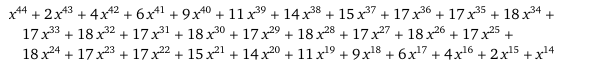
If we multiply two standard dice together:

$(x+x^2+x^3+x^4+x^5+x^6) * (x+x^2+x^3+x^4+x^5+x^6)$

We get the polynomial:

$x^2 + 2x^3 + 3x^4 + 4x^5 + 5x^6 + 6x^7 + 5x^8 + 4x^9 + 3x^{10} + 2x^{11} + x^{12}$

If you add up how many faces there are, that would be a 36 sided dice, and if you look at the number of faces of each value, you can see they follow the same binomial distribution that we showed in the problem statement section, when adding two dice together.

We aren’t done yet though, we need to see if there’s an alternate way to break this 36 sided dice polynomial back into two 6 sided dice, that aren’t just the standard 6 sided dice.

We need to factor that large polynomial into two smaller ones. These smaller polynomials have requirements (constraints) as well, to be valid:

Each $a_k$ needs to be non negative. That is, you can’t have a negative number of face values on a dice. That’d be weird.
The labels need to be positive. 0 is not a valid face value. This means that $a_0 = 0$ so that $a_0*x^0$ is 0.
The dice should have 6 faces. So if you sum up $a_k$ for all $k$ , it should give you 6.

The second bullet point can be described as $f(0) = 0$ because it makes all the $x$ power terms go away and leaves only the value of $a_0$ .

The third bullet point can be described as $f(1) = 6$ because that will make all $x$ power terms become 1, and so it will just be the $a_k$ values summed up.

The first step is to decompose the large polynomial into irreducible (prime) factors. In the video, instead of factoring the large polynomial, he factors the standard dice polynomial instead, and duplicates the factors, to get the list below. This video is a good intro to factoring polynomials if you need it: https://www.youtube.com/watch?v=KUMhpKGwpCY

$x$
$(1+x)$
$(1-x+x^2)$
$(1+x+x^2)$
$x$
$(1+x)$
$(1-x+x^2)$
$(1+x+x^2)$

To make new dice, we are going to assign each of those factors above to one of the dice. The factors assigned to a dice are going to be multiplied together to get the final polynomial for the dice.

We start with the second constraint that $f(0)=0$ . The only way that can be true is if each dice has the $x$ factor. So, we assign one of those to the first dice, and the other one to the second dice.

Dice A: $x$
Dice B: $x$

Let’s move onto the second constraint that $f(1)=6$ . If we plug 1 in for $x$ , the factor we already have for each dice evaluates to 1,and here are the values we get for each of the factors remaining:

$(1+x) = 2$
$(1-x+x^2) = 1$
$(1+x+x^2) = 3$
$(1+x) = 2$
$(1-x+x^2) = 1$
$(1+x+x^2) = 3$

Since we are multiplying factors together, and we need both of the dice to evaluate to 6, that means we assign $(1+x)$ to each dice to multiply by 2, and also assign $(1+x+x^2)$ to each dice to multiply by 3, so that we are multiplying each dice by 6.

Our dice are identical right now, looking like this:

Dice A: $x*(1+x)*(1+x+x^2)$
Dice B: $x*(1+x)*(1+x+x^2)$

We also have two factors left to assign:

$(1-x+x^2)$
$(1-x+x^2)$

If we gave each dice one of these factors, we’d end up at the standard dice again, so the idea is to give both factors to one of the dice to get this:

Dice A: $x*(1+x)*(1+x+x^2)$
Dice B: $x*(1+x)*(1+x+x^2)*(1-x+x^2)*(1-x+x^2)$

We can multiply these out to get the following polynomials:

Dice A: $x + 2x^2 + 2x^3+ x^4$
Dice B: $x + x^3 + x^4 + x^5 + x^6 + x^8$

Listing out the faces of the dice, we find we’ve made the Sicherman dice! Also, all three constraints are satisfied by both dice.

Dice A: 1, 2, 2, 3, 3, 4
Dice B: 1, 3, 4, 5, 6, 8

Explanation As Convolution

When I saw this, it made sense to me in terms of convolution. There are two concepts here to show what I mean.

The first concept is that if you add together two random values, you are also convolving their probability distributions. For discrete random values, such as dice, you are convolving their Probability Mass Function (PMF) which is a normalized histogram. For continuous random values, you are convolving their Probability Density Function (PDF). See this for more information: https://en.wikipedia.org/wiki/Convolution_of_probability_distributions

The second concept is that when you multiply polynomials together, you are actually doing convolution of their coefficients.

For instance, if you wanted to convolve the sequence 1,1 with the sequence 1,1 that would give you the sequence 1,2,1.

We can set this up with polynomials by giving each term in the sequence a unique power of x:

$f(x) = 1*x^0 + 1*x^1 = 1 + x$
$g(x) = 1*x^0 + 1*x^1 = 1 + x$
$h(x) = f(x)*g(x) = (1+x)(1+x) = (1+2x+x^2)$

You can see that the coefficients of the result are 1,2,1 and gave us the same answer as convolution.

As a more complex example to help show this works, let’s convolve 2,2 with 1,2,3,4. That should give us 2, 6, 10, 14, 8. (Here’s an online discrete convolution calculator: https://www.rapidtables.com/calc/math/convolution-calculator.html)

$f(x) = 2*x^0 + 2*x^1 = 2+2x$
$g(x) = 1*x^0 + 2*x^1 + 3*x^2 + 4*x^3 = 1 + 2x + 3x^2 + 4x^3$
$h(x) = f(x)*g(x) = (2+2x)(1 + 2x + 3x^2 + 4x^3) = 2+6x+10x^2+14x^3+8x^4$

We got our answer in the coefficients again: 2, 6, 10, 14, 8.

So, if we want to get the probability distribution of the sum of two dice, we know we need to convolve their distribution. By making the dice histogram into polynomials, we can multiply the polynomials to do the convolution, and get our resulting histogram. The polynomial then just needs to be factored into two polynomials that satisfy the dice validity constraints.

Viewed from this perspective, this method seems like a “hacky party trick”.

Interestingly though, the part about factoring a polynomial into smaller polynomials can be seen as deconvolution in this point of view. Deconvolution is a powerful thing, and kind of an advanced topic, but to bring it to something tangible, if you have a blurry image, and you know the kernel that blurred the image, deconvolution lets you get the unblurred source image back.

As we saw in this situation though, factoring a polynomial into two other polynomials multiplied together does not always give a unique solution, and it isn’t an easy process to find and enumerate the solutions. This is also true in deconvolution, unsurprisingly! There are multiple methods for doing deconvolution. This polynomial factoring is equivalent to just one of the methods.

Generating Functions Introduction

The other way I wanted to talk about this problem is from the point of view of generating functions, which generalize this creative use of exponents into a powerful mathematical tool. Generating functions allow you to abstract certain types of problems as polynomial multiplication.

A generating function is a polynomial just like the ones we’ve been looking at: a sum of powers of x multiplied by coefficients.

$a_0x^0 + a_1x^1 + a_2x^2 + ... + a_nx^n$

When looking at a specific term $a_kx^k$ , the $a_k$ value says how many ways there are to select the value $k$ .

Example 1 – AABB

We’ll work through 2 examples of making generating functions. I’m taking these directly from the video https://www.youtube.com/watch?v=fL2zQii4B5E.

If we have a single letter A that we can select or not, there is 1 way to select 0 elements, and 1 way to select 1 elements. That gives a generating function $1*x^0 + 1*x^1$ which simplifies to:

$1 + x$ .

If we have the letters AA, there is 1 way to select 0 elements, 1 way to select 1 element (because the As are identical to each other), and there is 1 way to select 2 elements. That gives the generating function:

$1 + x + x^2$

If we also have the letters BB, they have the same generating function:

$1 + x + x^2$

To get the generating function for AABB, we are selecting from AA and from BB and adding them together, so we multiply the generating functions together:

$(1 + x + x^2) * (1 + x + x^2)$

Which equals:

$1+2x+3x^2+2x^3+x^4$

That shows us there is:

1 way to select 0 elements
2 ways to select 1 elements (just A or just B)
3 ways to select 2 elements (AA, BB, AB)
2 ways to select 3 elements (AAB or ABB)
1 way to select 4 elements (AABB)

Example 2 – ABCD

Going back to a single letter choice, we can take the letter or leave it, giving us the generating function:

$1 + x$ .

If we have four letters we can choose from (or not) – ABCD – we multiply that generating function by itself four times: once per letter.

$(1 + x)*(1 + x)*(1 + x)*(1 + x)$

That equals:

$1 + 4x + 6x^2 + 4x^3 + x^4$

This shows us there is:

1 way to select 0 elements
4 ways to select 1 element (A, B, C or D)
6 ways to select 2 elements (AB, AC, AD, BC, BD, CD)
4 ways to select 3 elements (BCD, ACD, ABD, ABC)
1 way to select 4 elements (ABCD)

Fun fact: you may notice this is the 5th row of Pascal’s triangle. This relates to binomial expansion and the binomial theorem. This also relates to Bernouli trials, since we are either taking each letter or leaving it. This series of values is also is what happens if you convolve 1,1 against itself, four times!

Problem 1 – Summing Three Numbers

Let’s work through two simple problems to better understand the application of generating functions before talking about the dice problem. These examples come directly from this video https://www.youtube.com/watch?v=-drdeNMoe8w.

For the first problem, we want to know how many ways are there to sum three numbers to get an answer of 12, when each number is between 0 and 6 inclusively.

We want to know how many ways $A+B+C=12$ can be true, when $A,B,C \in [0,6]$ .

Choosing a number between 0 and 6 is represented by the generating function $(1 + x + x^2 + x^3 + x^4 + x^5 + x^6)$ . If we want to do that three times – once for A, once for B, once for C – and add them together, we multiply that generating function by itself three times, aka we cube it.

$(1 + x + x^2 + x^3 + x^4 + x^5 + x^6)^3$

That gives:

$1 + 3x + 6x^2 + 10x^3 + 15x^4 + 21x^5 + 28x^6 + 33x^7 + 36x^8 + 37x^9 + 36x^{10} + 33x^{11} + 28x^{12} + 21x^{13} + 15x^{14} + 10x^{15} + 6x^{16} + 3x^{17} + x^{18}$

The coefficient for $x^{12}$ is 28, which means there are 28 different ways to add the three numbers between 0 and 6 together, to get 12.

Problem 2 – Picking Jelly Beans

Imagine we have a jar of red, blue and white jellybeans. We want to know how many ways there are to select 20 jelly beans such that:

We have an even number of red jelly beans
We have at least 14 blue jelly beans.
We have less than 5 white jelly beans.

Those three constraints become these three generating functions:

$(1+x^2 + x^4 + ... + x^{20})$
$(x^{14}+x^{15}+ ... + x^{20})$
$(1 + x + x^2 + x^3 + x^4)$

The first and second generating functions could extend beyond $x^{20}$ into infinity, but we know there are 20 jellybeans total, so we can stop at 20.

Multiplying those three together gives us the polynomial below, which shows us that $x^{20}$ has a coefficient of 14. There are 14 different ways to select 20 jellybeans while satisfying the constraints.

Explanation As Generating Functions

Looking at the original dice summing problem from the perspective of generating functions, you can see that we have individual dice that have generating functions describing how many ways there are to roll each number.

With a standard 6 sided dice, the generating function only has one way to roll each number:

$1 + x + x^2 + x^3 + x^4 + x^5 + x^6$

For our modified dice where we replaced the 2 face with a 4, that meant there was no way to get a 2 anymore, but there were two ways to get a 4:

$1 + x + x^3 + 2x^4 + x^5 + x^6$

Multiplying dice polynomials together gave the histogram of how many ways each value could come up if you rolled two dice and added them together.

In the example problems of generating functions in the last section, we only concerned ourselves with a single coefficient, because we wanted to know how many ways a specific value could be selected.

In the dice summing problem though, we are concerned with ALL coefficients. The reason for this is because we are trying to get a specific histogram of possible selected values. A histogram is an array of counts, which is what the coefficients are. So, our dice problem is just a generating function problem which concerns itself with multiple coefficients. That’s still well within the realm of normality for generating functions.

The generating function point of view of this problem helps give a more formal footing to this method, rather than the “hacky party trick” point of view, but I don’t believe it helps you factor the final generating function of the summed dice into the two individual generating functions needed for the alternately labeled dice. It’s just another way of explaining why the polynomial shenanigans work.

Closing

If you’ve done any DSP work, as you learn more about generating functions you may notice they are pretty similar to the z transform (the discrete laplace transform). In generating functions, you can shift the index of the coefficient you need to calculate by multiplying by positive or negative powers of x, just like you can multiply by z to shift a sample in time. I have two write ups on the DSP side of things regarding this if you want to know more:

Here are the videos I found most helpful when learning about generating functions. Some of these were linked above in the article already FYI.

There is a method to get a single coefficient without having to calculate them all, using the Extended Binomial Theorem. That is explained in the second link above.

If you liked this post, you would probably also be interested in this post, which talks about summing discrete number sequences using something called “Umbral Calculus”: https://blog.demofox.org/2022/08/09/calculating-discrete-sums-with-umbral-calculus/

Thanks for reading, and hopefully you found this topic as interesting as I did!

Update: Someone shared some pretty cool posts about generating functions and dice for the board game “Arcs”:

The blog at the bottom of the sea

Programming, Graphics, Gamedev, Exotic Computation, Audio Synthesis

Monthly Archives: January 2025

Dice, (De)Convolution and Generating Functions